Today, we will start introducing physical operators in SQL Server. In the storage engine series, we touched on some of them, like index seek and scan. Here we will start with the simplest of them, scalar aggregates. Now, in SQL Server, there are two of them:

Stream
and Hash aggregate

These two are used to perform various types of aggregations

So, what is an aggregation?

It is a way of summarising some information about a subset of data, like the COUNT() or the standard deviation

So you get the information you want, like what is the MAX in employee salary, etc.

Table of Contents

Intro

So, what is a scalar aggregate? It's the type of aggregate that returns one value and does not have a group by clause, meaning it uses the whole column, table as a group, instead of another definition like employeeid

Now, how does SQL Server implement them? using the physical operator stream aggregate

For example:

use AdventureWorks2022
go
select count(*) from Production.Product
go

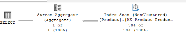
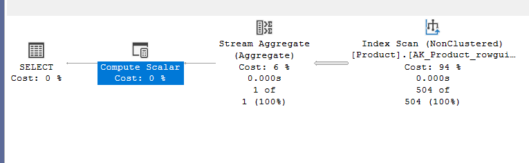
The output was 504, and the execution plan:

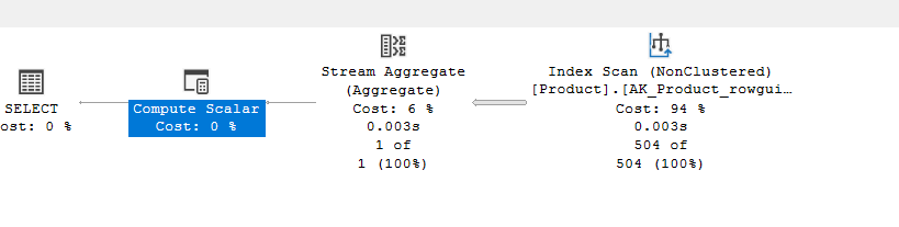
So the stream aggregate here is our aggregation

The index scan is to get the data to count it

The compute scalar it to convert the output of the stream aggregate to from bigint to int since count()’s output is in INT. Now we can get rid of it by using count_big()(more on both is coming), , and the select is our logical select operator

No,w if we dive into the properties of the aggregate:

Graphical plan

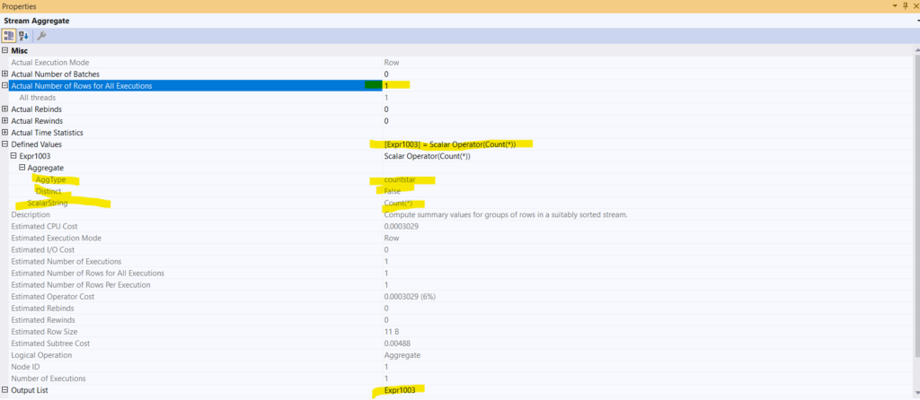
So, as we can see here and in the output of the query, the number of rows is one, since there is only one count for the number of rows in the table

The logical operator is an aggregate scalar operator that deals with simple mathematical calculations(different than the scalar aggregate itself, more on it in our logical tree generation blog) that counts the rows in the table, and the string is count(*), like we wrote

The output of it is stored in the expr1003, and this is what the operator result is, and it is in bigint, this is why we need the upcoming compute scalar

And it is implemented using the Stream aggregate physical operator

In the properties of the compute scalar:

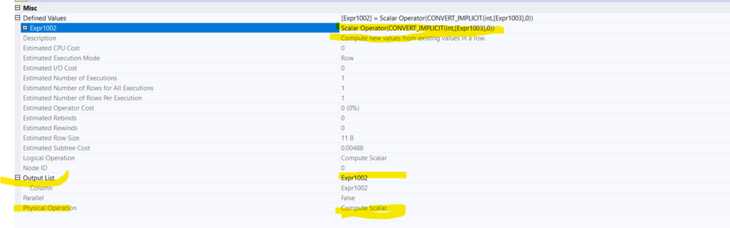
So it converts the output of the stream aggregate function, which returns bigint values to int

Now the textual plan:

Textual plan

If we execute the following:

use AdventureWorks2022;
go
set showplan_text on; 
go
select count(*) from Production.Product
go
set  showplan_text off ; 
go

We get:

  |--Compute Scalar(DEFINE:([Expr1002]=CONVERT_IMPLICIT(int,[Expr1003],0)))
    |--Stream Aggregate(DEFINE:([Expr1003]=Count(*)))
      |--Index Scan(OBJECT:([AdventureWorks2022].[Production].[Product].[AK_Product_rowguid]))

You can see what we saw before, an index scan and the defined accessed object, which is the index

The stream aggregate, and the convert_implicit compute scalar

For the XML:

XML plan:

For the index scan:

  <RelOp 
  AvgRowSize="....
  lSubtreeCost="0.00457714" TableCardinality="504">
    <OutputList />
    <RunTimeInformation>
      <RunTimeCountersPerThread 
      T.........
    </RunTimeInformation>
    <IndexScan 
.......>
  <DefinedValues />
  <Object
   Database="[AdventureWorks2022]" 
   Schema="[Production]" 
   Table="[Product]" 
   Index="[AK_Product_rowguid]" 
   IndexKind="NonClustered" 
   Storage="RowStore" />
</IndexScan>
  </RelOp>

Here we see the same stuff we saw before in the graphical plan

For the stream aggregate:

<RelOp 
.....>
  <OutputList>
    <ColumnReference Column="Expr1003" />
  </OutputList>
  <RunTimeInformation>
    <RunTimeCountersPerThread.....
  </RunTimeInformation>
  <StreamAggregate>
    <DefinedValues>
      <DefinedValue>
        <ColumnReference Column="Expr1003" />
        <ScalarOperator ScalarString="Count(*)">
          <Aggregate AggType="countstar" Distinct="false" />
        </ScalarOperator>
      </DefinedValue>
    </DefinedValues>
  
  </StreamAggregate>
</RelOp>

Here we see what we saw before, the expr1003

We can see that the distinction is false, same as the graphical plan(more on this later in this blog)

Other than that, we don’t see much.

For the compute scalar:

<RelOp ......
              
              <OutputList>
                <ColumnReference Column="Expr1002" />
              </OutputList>
              <ComputeScalar>
                <DefinedValues>
                  <DefinedValue>
                    <ColumnReference Column="Expr1002" />
                    <ScalarOperator ScalarString="CONVERT_IMPLICIT(int,[Expr1003],0)">
                      <Convert DataType="int" Style="0" Implicit="true">
                        <ScalarOperator>
                          <Identifier>
                            <ColumnReference Column="Expr1003" />
                          </Identifier>
                        </ScalarOperator>
                      </Convert>
                    </ScalarOperator>
                  </DefinedValue>
                </DefinedValues>
                
              </ComputeScalar>
            </RelOp>

Now, here we see the convert_implicit. And it's expr1002, and it is getting the expr1003.

Other than that, not much here either.

Now, for completeness’s sake, we are going to get rid of the compute scalar:

use AdventureWorks2022
go
select count_big(*) from Production.Product
go

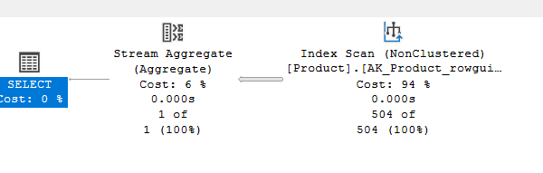
So no compute scalar.

But what would happen when we don’t have rows to output like:

use AdventureWorks2022;
go
create table tabl(
id int null
)
select count(*) from tabl
go

The output was like:

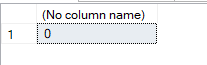
So 0, which, as Craig Freedman and Conor Cunningham say, is the only nonleaf operator that produces output even when there are no rows, meaning the stream aggregate, same happens with other aggregate functions like sum(), which has huge implications on indexed views that we will discuss in another blog

0 is a value, not empty.

Now the next section is a little bit advanced, so you can skip it if you like we introduced it here

Logical tree generation

If we run the following:

use adventureworks2022;
go
dbcc traceon(3604);
go

select count(*)
from production.product
option (recompile, querytraceon 8605, querytraceon 8606, querytraceon 8607,
        querytraceon 8608, querytraceon 8621, querytraceon 3604,
        querytraceon 8620, querytraceon 8619, querytraceon 8615,querytraceon 8675, querytraceon 2372);
go

Now we are going to choose the relevant parts:


*** Converted Tree: ***
LogOp_Project COL: Expr1002 

   LogOp_GbAgg OUT(COL: Expr1002 ,)

     LogOp_Get TBL: production.product production.product TableID=162099618 TableReferenceID=0 IsRow: COL: IsBaseRow1000 

     AncOp_PrjList 

          AncOp_PrjEl COL: Expr1002 

              ScaOp_AggFunc stopCount Transformed

                ScaOp_Const TI(int,ML=4) XVAR(int,Not Owned,Value=0)

        AncOp_PrjList

So, here:

LogOp_Project COL: Expr1002: here the projection operator is like a select clause, meaning it will get all the rows from the Expr1002, which, as we know now, is the compute scalar physical operator output, it has 2 child operators:
- LogOp_GbAgg OUT(COL: Expr1002,): now, here it is simply saying we have an aggregation, and it should output this expression, it has 2 child operators:
  - LogOp_Get TBL: which only gets the rows from the provided definition
  - AncOp_PrjList: which does what we want, includes aggregates, computed columns, etc., it has 1 child operator:
    - ScaOp_AggFunc stopCount Transformed: So here it defines that it wants a scalar logical operator that deals with simple math, which is the COUNT. Now it is going to define the structure of the output of the count, one child operator, which is the scop_const

For the physical output plan:

*** Output Tree: (trivial plan) ***

        PhyOp_StreamGbAgg( )

            PhyOp_NOP

                PhyOp_Range TBL: production.product(4) ASC  Bmk ( QCOL: [AdventureWorks2022].[Production].[Product].ProductID) IsRow: COL: IsBaseRow1000 

            AncOp_PrjList 

                AncOp_PrjEl COL: Expr1002 

                    ScaOp_AggFunc stopCount Transformed

                        ScaOp_Const TI(int,ML=4) XVAR(int,Not Owned,Value=0)

********************

So we have the streamagg physical operator that gets through scanning the values from the table where the range operator lies, while aggregating

Nothing new here, other than the fact that I can’t see the compute scalar for the convert_implicit?

Now the same structures would show with any other scalar aggregation like MIN()

Using the same stream aggregate for multiple calculations

For example:

use AdventureWorks2022
go
select max(p.ProductNumber),min(p.ProductNumber)
from Production.Product p
go

We get:

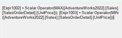
If we look at the properties:

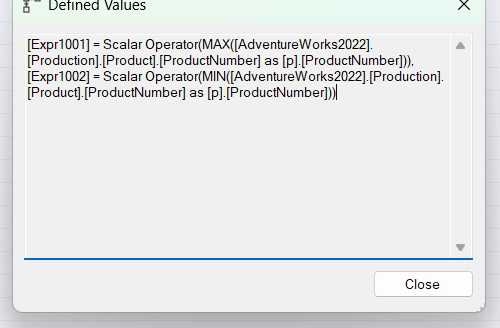
So, as you can see, it calculates both, minimum and maximum, and there is no convert implicit, since the aggregation in max and min is based on the datatype of productnumber

The textual execution plan:

  |--Stream Aggregate(DEFINE:([Expr1002]=**MAX**([AdventureWorks2022].[Production].[Product].[ProductNumber]), 
  [Expr1003]=**MIN**([AdventureWorks2022].[Production].[Product].[ProductNumber])))
       |--Index Scan(OBJECT:([AdventureWorks2022].[Production].[Product].[AK_Product_ProductNumber]))

In the XML:

   <OutputList>
      <ColumnReference Column="Expr1002" />
      <ColumnReference Column="Expr1003" />
    </OutputList>
    <StreamAggregate>
    
 <ColumnReference Column="Expr1002" />
<ScalarOperator ScalarString="MAX([AdventureWorks2022].[Production].[Product].[ProductNumber])">
 <Aggregate AggType="MAX" Distinct="false">
  <ScalarOperator>
     <Identifier>
   <ColumnReference Database="[AdventureWorks2022]" Schema="[Production]" Table="[Product]" Column="ProductNumber" />
               
  <ColumnReference Column="Expr1003" />
   <ScalarOperator ScalarString="MIN([AdventureWorks2022].[Production].[Product].[ProductNumber])">
   <Aggregate AggType="MIN" Distinct="false">
             
   <ColumnReference Database="[AdventureWorks2022]" Schema="[Production]" Table="[Product]" Column="ProductNumber" />
                
    </StreamAggregate>
  </RelOp>

AVG as a scalar aggregate:

Now, if we do the following:

use AdventureWorks2022
go
select avg(TaxAmt)from Sales.SalesOrderHeader
go

The graphical:

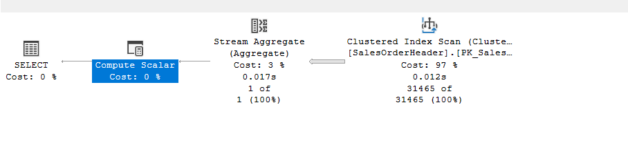
The scan is the scan

The stream aggregate properties:

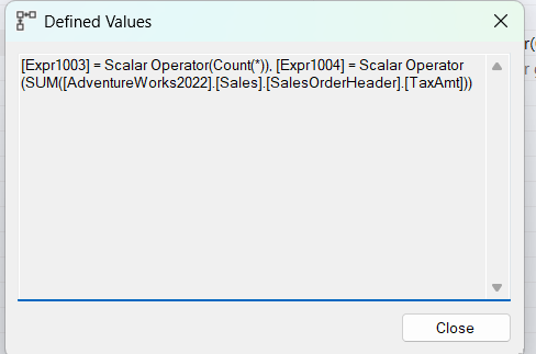
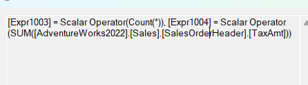
So here it is, defining and aggregating like it did in the min and max combined, a count() and a sum() for the division

Then, in the compute scalar:

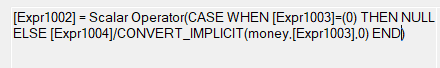
The case when is for avoiding dividing by 0, so when count = 0, then don’t divide and output null(more on this in another blog), otherwise calculate our avg and output as expr1002

The textual:

  |--Compute Scalar(DEFINE:([Expr1002]=CASE WHEN [Expr1003]=(0) 
  THEN NULL ELSE [Expr1004]/CONVERT_IMPLICIT(money,[Expr1003],0) END))
       |--Stream Aggregate(DEFINE:([Expr1003]=Count(*), 
       [Expr1004]=SUM([AdventureWorks2022].[Sales].[SalesOrderHeader].[TaxAmt])))
            |--Clustered Index Scan(OBJECT:([AdventureWorks2022].[Sales].[SalesOrderHeader].[PK_SalesOrderHeader_SalesOrderID]))

Nothing much,

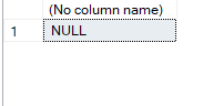
Now, what would happen when we have 0 rows:

use adventureworks2022
go
select avg(id) from tabl
go

So, it would always provide one output, no matter what, even when there is nothing, not null, which is not nothing.

SUM as a scalar aggregate:

So:

use AdventureWorks2022
go
select sum(TaxAmt)from Sales.SalesOrderHeader
go

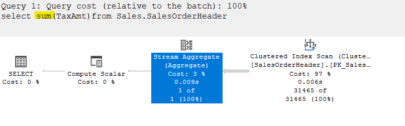
In the properties of the aggregate:

So even though we don’t need the count(*) here, it used that to prevent the division by null

In the compute scalar:

So when count(*) is 0, then null, otherwise output the expr1004 which is our sum only, not the division

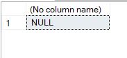
Now, if we sum in an empty table:

use adventureworks2022
go
select sum(id) from tabl
go

as expected.

Scalar DISTINCT

Now what would happen if we add distinct in the count:

use adventureworks2022
go
select count(distinct(Class)) from production.product
go

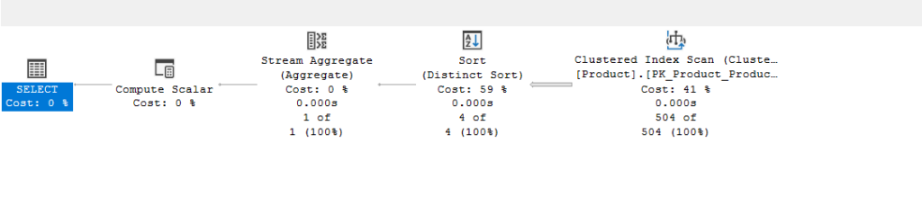
Now if we look at the properties of the distinct sort:

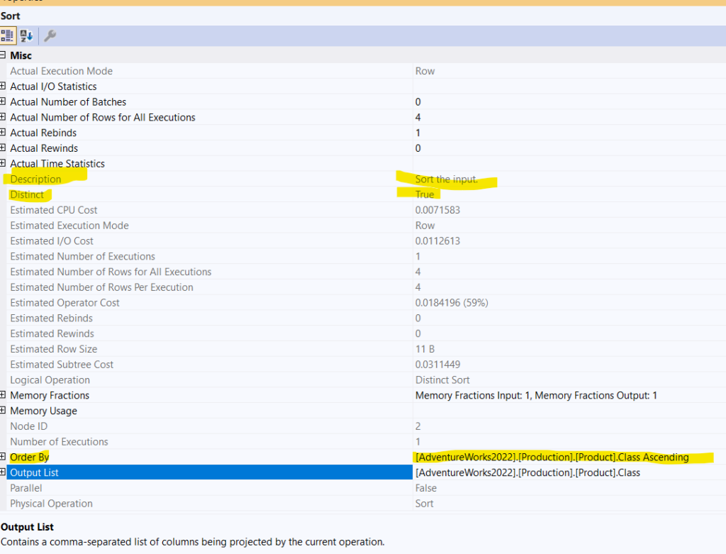
So, we have an order by that we did not ask for excplictly, but it did it to arrange the values neatly next to each other so it could eliminate duplicates, since distinct is just sort and kick out the duplicates, after that it kicked out the duplicates by distinct true

Other than that, the plan is the same as the count(*) plan

The textual:

|--Compute Scalar(DEFINE:([Expr1002]=CONVERT_IMPLICIT(int,[Expr1005],0)))
 |--Stream Aggregate(DEFINE:([Expr1005]=COUNT([AdventureWorks2022].[Production].[Product].[Class])))
   |--**Sort**(**DISTINCT** **ORDER BY**:([AdventureWorks2022].[Production].[Product].[**Class**] **ASC**))
     |--Clustered Index Scan(OBJECT:([AdventureWorks2022].[Production].[Product].[PK_Product_ProductID]))

What about distinct with other aggregate functions:

Distinct with max and min

Like the following:

use adventureworks2022
go
select 
max(distinct(UnitPrice)),min(distinct(UnitPrice))
from 
Sales.SalesOrderDetail
go

We get:

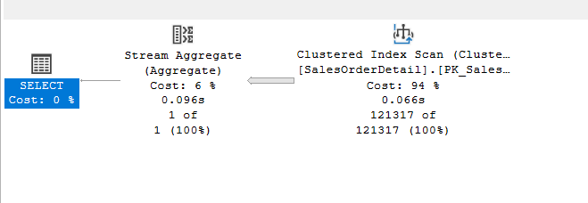
The same plan as the plan before, the one without the distinct:

So, no distinct

Distinct on a unique key

like:

use adventureworks2022
go
select count(distinct(name)) from production.product
go

the plan was like:

So no sort, since every row is unique in name in production.product as we can see here

Now could we see that in action:

use adventureworks2022;
go
dbcc traceon(3604);
go

select count(distinct(name)) from production.product

option (recompile, querytraceon 8605, querytraceon 8606, querytraceon 8607,
        querytraceon 8608, querytraceon 8621, querytraceon 3604,
        querytraceon 8620, querytraceon 8619, querytraceon 8615, querytraceon 2372);
go

In the converted tree:

*** Converted Tree: ***
    LogOp_Project COL: Expr1002 

        LogOp_GbAgg OUT(COL: Expr1002 ,)

            LogOp_Get TBL: production.product production.product TableID=162099618 TableReferenceID=0 IsRow: COL: IsBaseRow1000 

            AncOp_PrjList 

                AncOp_PrjEl COL: Expr1002 

                    **ScaOp_AggFunc stopCount Distinct Transformed**

                        ScaOp_Identifier QCOL: [AdventureWorks2022].[Production].[Product].Name

        AncOp_PrjList 

*******************

The only new thing here is that the aggregate function, which is the distinct aggregate logical operator

But we see this in the output:

NormalizeGbAgg transformation rule:

***** Rule applied: NormalizeGbAgg - Gb(a,b,c) sum(b) -> Gb(a,b) any(c), sum(b)

    LogOp_GbAgg OUT(COL: Expr1002 ,)

      LogOp_Get TBL: production.product production.product TableID=162099618 TableReferenceID=0 IsRow: COL: IsBaseRow1000 

      AncOp_PrjList 

        AncOp_PrjEl COL: Expr1002 

          **ScaOp_AggFunc stopCount**

            ScaOp_Identifier QCOL: [AdventureWorks2022].[Production].[Product].Name

***** Rule applied: NormalizeGbAgg - Gb(a,b,c) sum(b) -> Gb(a,b) any(c), sum(b)

    LogOp_GbAgg OUT(COL: Expr1002 ,)

      LogOp_Get TBL: production.product production.product TableID=162099618 TableReferenceID=0 IsRow: COL: IsBaseRow1000 

      AncOp_PrjList 

        AncOp_PrjEl COL: Expr1002 

          ScaOp_AggFunc stopCount

            **ScaOp_Const TI(int,ML=4) XVAR(int,Not Owned,Value=0)**

So here it looked, it found that the index is unique, so it replaced it with a regular count

Then, it applied the rule again, since it realized that the output of count, unlike sort distinct, is a constant scalar int

This plan is trivial, meaning these rules of transformation are almost free to execute

Multiple distincts

Now what if we had two DISTINCT in the same query:

use adventureworks2022
go
select count(distinct(productline)),
       count(distinct(class))
from production.product
go

In the next blog, since there are a lot of transformation rules that could be useful here.

Intro

Graphical plan

Textual plan

XML plan:

Logical tree generation

Using the same stream aggregate for multiple calculations

AVG as a scalar aggregate:

SUM as a scalar aggregate:

Scalar DISTINCT

Distinct with max and min

Distinct on a unique key

NormalizeGbAgg transformation rule:

Multiple distincts

Leave a Reply Cancel reply

Quick Links

Get In Touch