
Today, we are going to introduce the first physical join operator. There are three operators: nested loop, hash, and merge join.
There is a mix between nested and hash = the adaptive join operator.
intro
In the join operator, we have two tables, the inner and the outer tables
The outer table is at the top = left table = outer input
The inner table is the one below = right table = inner input
We can see that if we do the following:
use AdventureWorks2022
go
select *
from Sales.SalesPerson sp inner join Sales.SalesPersonQuotaHistory sph on sph.BusinessEntityID = sp.BusinessEntityID
where sp.BusinessEntityID < 275
go
We get:
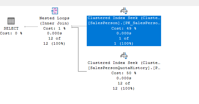
The upper is the outer,
The algorithm
It compares each row from the first input, the outer one, to the inner input, one by one, and sees if they match the predicate we specified
The pseudo-code for this by Craig Freedman :
for each row R1 in the outer table
for each row R2 in the inner table
if R1 joins with R2
return (R1, R2)
So it glues each row that matches with the other one, meaning it nests them, and that is why it is called a nested loop join.
The more rows you have, the more you nest, the more it costs
Now, each row in the outer table is compared to each inner output until it finds a match for it
So the more the outer, the more the inner has to be scanned again and again until it finds a match for the row in question
Also, the more inner row, the more you have to scan for each outer table we try to match to
So the cost increases too much due to the increase in the size of the inner
But, what if we have an index on the inner input? Then we only look up the rows we need so quickly and compare them
So if we have a small set of rows in the outer input, and we have an index on the inner input, then the cost is cheap
But if we need a table scan each time we compare, it is going to take forever for each row
So if we had two tables like:
use adventureworks2022
go
create table table1 (
    id int,
    col11 int
);

create table table2 (
    id int,
    col12 int
);

insert into table1 (id, col11) values (3, 45);
insert into table1 (id, col11) values (12, 87);
insert into table1 (id, col11) values (7, 23);
insert into table1 (id, col11) values (18, 91);
insert into table1 (id, col11) values (5, 14);
insert into table1 (id, col11) values (9, 62);
insert into table1 (id, col11) values (22, 33);
insert into table1 (id, col11) values (14, 78);
insert into table1 (id, col11) values (8, 19);
insert into table1 (id, col11) values (25, 55);
insert into table1 (id, col11) values (11, 42);
insert into table1 (id, col11) values (6, 67);
insert into table1 (id, col11) values (19, 88);
insert into table1 (id, col11) values (2, 29);
insert into table1 (id, col11) values (10, 73);
insert into table1 (id, col11) values (4, 37);
insert into table1 (id, col11) values (17, 50);
insert into table1 (id, col11) values (23, 64);
insert into table1 (id, col11) values (15, 81);
insert into table1 (id, col11) values (1, 95);

insert into table2 (id, col12) values (7, 12);
insert into table2 (id, col12) values (5, 30);
insert into table2 (id, col12) values (18, 44);
insert into table2 (id, col12) values (3, 99);
insert into table2 (id, col12) values (9, 27);
insert into table2 (id, col12) values (12, 68);
insert into table2 (id, col12) values (20, 53);
insert into table2 (id, col12) values (6, 76);
insert into table2 (id, col12) values (14, 39);
insert into table2 (id, col12) values (8, 61);
insert into table2 (id, col12) values (1, 84);
insert into table2 (id, col12) values (22, 17);
insert into table2 (id, col12) values (19, 72);
insert into table2 (id, col12) values (10, 48);
insert into table2 (id, col12) values (4, 25);
insert into table2 (id, col12) values (25, 90);
insert into table2 (id, col12) values (13, 59);
insert into table2 (id, col12) values (2, 66);
insert into table2 (id, col12) values (7, 31);
insert into table2 (id, col12) values (11, 78);
go
Now, if we join like:
select*
from table1 t1 inner loop join table2 t2 on t1.id = t2.id;
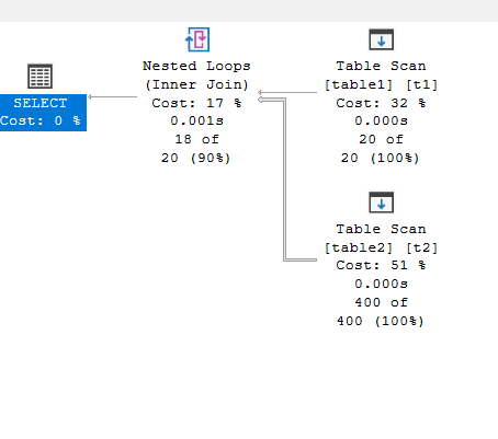
So we have 20 rows in the first, and for each we ran the second 20 20 times = 400 to get the result, which was estimated to be 20
Now, so the cost is based on the cost of producing the outer rows, multiplied by the cost of producing the inner rows for each outer row, if we had an index, sometimes it would be an index seek for that specific outer row
For example:
go
create table new1
(
id int,
col1 varchar(20)
)
insert into new1 values(1,'a'),(2,'b'),(3,'c')
create table new2 ( id int, col1 varchar(20))
insert into  new2 values (2,'b'),(2,'c'),(3,'d')

go
select*
from new1 inner loop join new2 on new1.id = new2.id
We get:
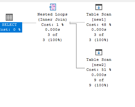
So it did the same here, but what if we had an index like:
create clustered index ix_n on new2(id)
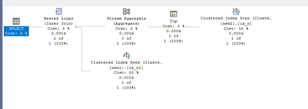
Then run the same query:
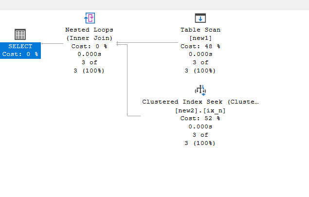
So, we reduced it to the third, since it only had to look for the matching predicate, so this is how we could reduce the cost of a nested loop join
Now, if we look at the tooltip:
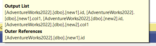
We can see the join predicate we specified, and we can see the outer references property, meaning the seeks we got from the ix_n were depending on the new1. id as a parameter for the seek
So id here is a correlated parameter for the join.
This is what you call an index join.
Now obviously, if we had to seek too much to get it, then there is no point in the index and the nested loop join becomes inefficient.
Join predicates supported by the nested loop join.
Since the fallback of any join is a nested loop join, it can support all kinds of predicates, like equality, as we saw, inequality, like:
select*
from new1
where new1.id >(select min(id) from new2)
No other join physical operator supports this
What about logical join operations
all of them except for:
- Right and full outer join
- Right semi-join and right anti-semi-join
Why does it not do that?
Efficiency,
If we try to left outer join, we would just output null for the rows that do not match where we don’t have a predicate matching
But what would happen if we try to right outer join: we would have to scan the inner table multiple times for each outer row, and then output 1 after a full scan of the inner input each time, which would make it very expensive
Now, obviously, a right outer join is commutative with a left one, but once we do this transformation, we decrease the amount of rules that could be used for that specific query, making for less optimal plans
What about full outer joins?
We can’t do it with a nested loop directly, but the optimizer can rewrite it, so if we do the following:
select*
from new1 full outer loop join new2 on new2.id = new1.id;
We get:
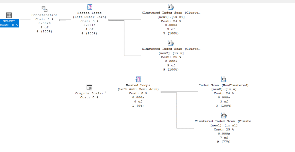
So we see 4 index scans, two nested loop joins, and one concat
The concat = union or union all
Now I created some indexes on the tables while making this demo, so you might not get the exact same result
In the tooltips of the lower nested loop join:
Now, first it is a left anti-semi join
So, it equals = not exists
The outer input is the id of the new2 with col1, so it outputs the col1 in new1 where they don’t exist in the new1 table:
select *
from new2
where  not exists
(select 1
from new1
where new1.id = new2.id
)
If we execute it, we would get the same lower section, the compute scalar just stores the rows for us,
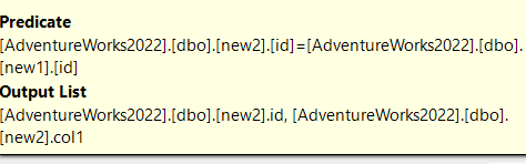
Now, in the tooltip of the second nested loop join:
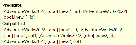
The same matching row, it is a left outer join, as you can see in the execution plan:
select*
from new1 left outer join new2 on new1.id = new2.id
If you do that, you would get the upper section
The concat is the union, so the query is:
select *
from new2
where  not exists
(select 1
from new1
where new1.id = new2.id
)
union
select*
from new1 left outer join new2
on new1.id = new2.id
Now, if you try to run this, you can’t, since the columns don’t match, but the execution plan properties have them, but this is basically what it did, this is obviously a huge move around the original query, which means more transformations between the original logical query and the physical implementation, meaning more cardinality estimation errors = slower performance
And this can’t scale.
With that, we finish our intro to nested loops, catch in the next one.