
In the previous blog, we stopped at that, today we are going to see how it gets executed, spoiler: it just does two separate distincts and then glues them. Here we are going to play with some trace flags, too see how this simple query got to this stage, the point here is to get an idea of how the parallel plan was disregarded, and see that in action, and give an example of the alternatives.
The Query
use adventureworks2022
go
select count(distinct(productline)),
       count(distinct(class))
from production.product
go
We get:
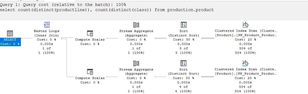
How did it combine these two aggregations? The answer is: it did not
It asked for a sort for each, like we see
aggregated separately
Then it cross-joined them, meaning joined them with no filtering predicate
meaning it just glued them together with a nested loop join
And how do we know that?
In the properties of the first sort distinct:
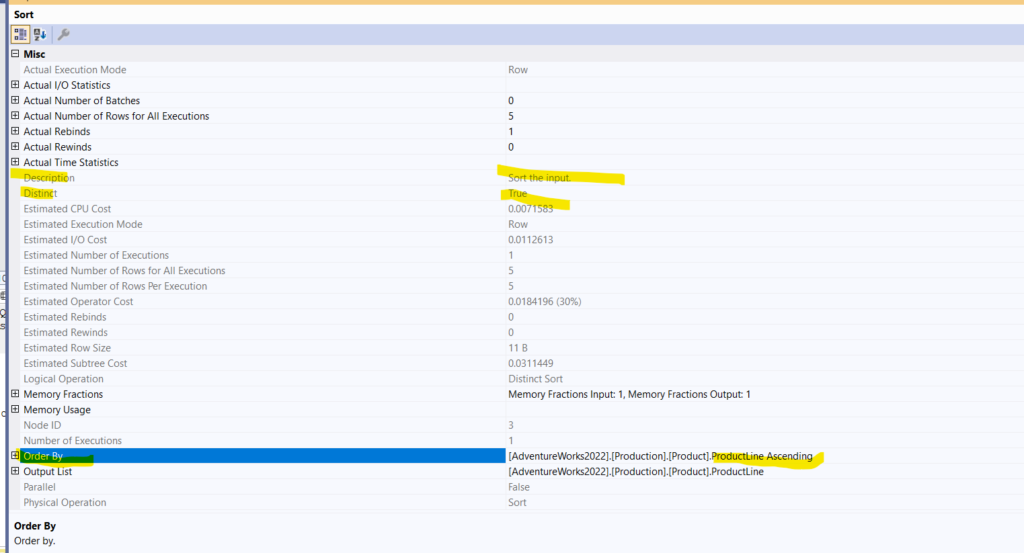
So it sorted based on the input, based on the productline, Ascending, nothing new here, then with the distinct, it removed the duplicates
The stream aggregate counts
And the compute scalar convert_implicit to int, like we showed in the previous blog
The second line does the same
But when we look at the properties of the nested loop join:
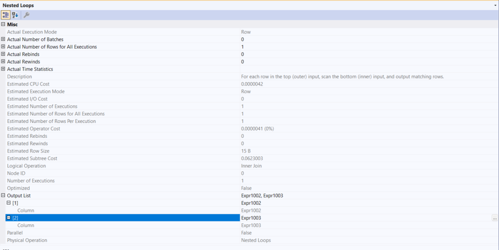
We are going to talk about the join operator in another blog, but as you can see, there is no join predicate, nor did we specify anything before this in an on or the old-fashioned way joining in a where clause.
So what do you call it when you don’t have filter predicates? a cross-join
But since all the rows from each are one, there is only one possible combination of cross-joining them
Meaning, all that the nested loop did was glue the two counts to each other
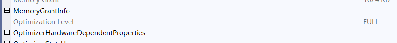
Now, this query was fully optimized, as you can check in the select properties like:
Now, if we look at the textual plan like:
use AdventureWorks2022;
go
set showplan_text on ;
go
select count(distinct(productline)),
       count(distinct(class))
from production.product
go
set showplan_text off;
go
We get:
|--Nested Loops(Inner Join)
     |--Compute Scalar(DEFINE:([Expr1002]=CONVERT_IMPLICIT(int,[Expr1008],0)))
     |    |--Stream Aggregate(DEFINE:([Expr1008]=COUNT([AdventureWorks2022].[Production].[Product].[ProductLine])))
     |         |--Sort(DISTINCT ORDER BY:([AdventureWorks2022].[Production].[Product].[ProductLine] ASC))
     |              |--Clustered Index Scan(OBJECT:([AdventureWorks2022].[Production].[Product].[PK_Product_ProductID]))
     |--Compute Scalar(DEFINE:([Expr1003]=CONVERT_IMPLICIT(int,[Expr1009],0)))
          |--Stream Aggregate(DEFINE:([Expr1009]=COUNT([AdventureWorks2022].[Production].[Product].[Class])))
               |--Sort(DISTINCT ORDER BY:([AdventureWorks2022].[Production].[Product].[Class] ASC))
                    |--Clustered Index Scan(OBJECT:([AdventureWorks2022].[Production].[Product].[PK_Product_ProductID]))
We can see the operators here more clearly next to each other, it sorts distinct, counted, then converted, after that it nests them together.
nothing much in the XML
Logical Tree generation
Now, before we look at the traces, we should mention sys.dm_exec_query_transformation_stats, now this is an undocumented cumulative DMV that shows all the transformation rules that has been implemented since the restart of the server, we introduced here. here we are going to take some snapshots of the query before and after the query, so we could know what the optimizer did
After that, we are going to run the traces and show the relevant information:
go
USE AdventureWorks2022;
go
BEGIN TRAN
SELECT *
INTO AFTER_TRANSFORMATION
FROM sys.dm_exec_query_transformation_stats;
COMMIT TRAN

BEGIN TRAN
SELECT *
INTO BEFORE_TRANSFORMATION
FROM sys.dm_exec_query_transformation_stats;
COMMIT TRAN

BEGIN TRAN
DROP TABLE AFTER_TRANSFORMATION;
DROP TABLE BEFORE_TRANSFORMATION;
COMMIT TRAN

BEGIN TRAN
SELECT *
INTO BEFORE_TRANSFORMATION
FROM sys.dm_exec_query_transformation_stats;
COMMIT TRAN

select count(distinct(productline)),
       count(distinct(class))
from production.product
where 1 = (select 1)
option(recompile);
BEGIN TRAN
SELECT *
INTO AFTER_TRANSFORMATION
FROM sys.dm_exec_query_transformation_stats;
COMMIT TRAN

BEGIN TRAN;
SELECT
    AFTER_TRANSFORMATION.name,
    (AFTER_TRANSFORMATION.promised - BEFORE_TRANSFORMATION.promised) AS PROMISED
FROM
    BEFORE_TRANSFORMATION
JOIN
    AFTER_TRANSFORMATION ON BEFORE_TRANSFORMATION.name = AFTER_TRANSFORMATION.name
WHERE
    BEFORE_TRANSFORMATION.succeeded <> AFTER_TRANSFORMATION.succeeded;
COMMIT TRAN;
go
We get:
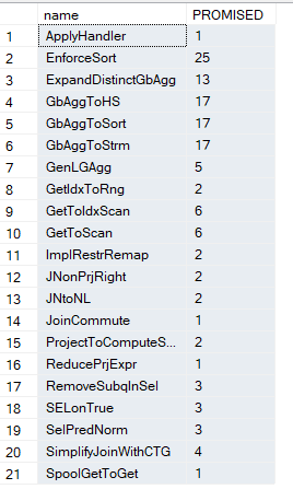
Now:
- Enforce sort is to force the sort in the distinct sort
- ExpandDistinctAggregate: is to expand each of the distinct logical operators to a sort and a distinct
- GbAggToHs, Sort, Strm: whether we should convert the logical aggregate to any of the following, is it a sort, hash, or a stream aggregate, obviously, the stream was applied here,
- GenLGAgg: generate local-global aggregate, now for more information on this rule you can check out SqlServerFast blog, but basically it means, make the parent(global) aggregate easier to calculate through different methodologies, using local aggregates, like you do with parallel plans by dividing the work between different child operators, then combining all in one aggregate, or by pre-aggregating some, we are going to detail this later in this blog
- GetIndToRng: so here it specifies what physical operator should be used on the index, like range scan
- GetIdxToScan: here it means scan, so in our plan it chose this, we are going to show the memo in a bit
- ImplRestrRemap: Implement restriction remapping. We are going to see it in action, in a bit, but here it eliminated the where 1 = (select 1 )
- JNonPrjRight: here it deletes the filters in the join predicate in the right, in a bit
- JNtoNL: converts the logical join to a nested loop join
- JoinCommute: uses the commutivity rule in relational algebra and applies it to joins where a join b = b join a etc.
- ProjectToComputeScalar: obvious
- ReducePrjExpr: gets rid of some of the generated expressions
- RemoveSubqInSel: it removes the subquery, it could be our 1 =(select 1 )
- SELonTrue: to remove redundant where clauses like 1 = 1
- SelPreNor: same
- SimplifyJoinWithCTG: could pull some predicates above joins
- SpoolGetToGet: now spools could be sometimes applied to aggregates, here it was considered and discarded.
Now, if we run without 1 = (select) we get the following:
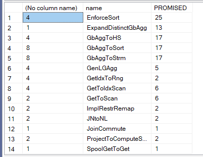
A lot of the rules for the 1 = ( select 1), so we are going to focus on those
Traces:
If we do the following:
use adventureworks2022;

go
dbcc traceon(3604);
go

select count(distinct(productline)),
       count(distinct(class))
from production.product
option (recompile, querytraceon 8605, querytraceon 8606, querytraceon 8607,
        querytraceon 8608, querytraceon 8621, querytraceon 3604,
        querytraceon 8620, querytraceon 8619, querytraceon 8615,querytraceon 8675, querytraceon 2372);
go
We get:
*** Tree After Project Normalization ***
        LogOp_GbAgg OUT(COL: Expr1002 ,COL: Expr1003 ,)

            LogOp_Get TBL: production.product production.product TableID=162099618 TableReferenceID=0 IsRow: COL: IsBaseRow1000

            AncOp_PrjList

                AncOp_PrjEl COL: Expr1002

                    ScaOp_AggFunc stopCount Distinct Transformed

                        ScaOp_Identifier QCOL: [AdventureWorks2022].[Production].[Product].ProductLine

                AncOp_PrjEl COL: Expr1003

                    ScaOp_AggFunc stopCount Distinct Transformed

                        ScaOp_Identifier QCOL: [AdventureWorks2022].[Production].[Product].Class

****************************************
Now, until Tree After Project Normalization, there is not much difference in the logical tree, if we try to explain it:
- LogOp_GbAgg OUT: outputs the aggregate not much 2 child operators one for the definition of the table to get from, and the other for computing what we want like the aggregates
- The first child of AncOp_PrjList is for the productline and the second is for the second
Now the initial memo:
Root Group 8: Card=1 (Max=1, Min=1)
   0 LogOp_GbAgg 0 7 (Distance = 0)
Group 7:
   0 AncOp_PrjList  3 6 (Distance = 0)
Group 6:
   0 AncOp_PrjEl  5 (Distance = 0)
Group 5:
   0 ScaOp_AggFunc  4 (Distance = 0)
Group 4:
   0 ScaOp_Identifier  (Distance = 0)
Group 3:
   0 AncOp_PrjEl  2 (Distance = 0)
Group 2:
   0 ScaOp_AggFunc  1 (Distance = 0)
Group 1:
   0 ScaOp_Identifier  (Distance = 0)
Group 0: Card=504 (Max=10000, Min=0)
   0 LogOp_Get (Distance = 0)
Now, here we put it as a reference to understand the rules while transforming. The group operator that references another number means that it references the other group in the same memo
For example, group 0 does not reference anything, it just represents LogOp_Get, but group 8 references 0 and 7, meaning the AncOp_Prjlist and LogOp_get, just the first parent operator in the tree, so it summarizes the tree in integers to reduce computational power used
Now, for the rules:
Apply Rule: ExpandDistinctGbAgg - Gb sum(dist d), sum(e) -> join(gb sum(e), gb dist sum(e))
    Args: Grp 8 0 LogOp_GbAgg 0 7 (Distance = 0)
So here it expanded the aggregates that is referenced by the parent operators group 8 operator number 0 which has the child operators in it 0 and 7, so here it created our logical sorts
The result:
Rule Result: group=8 1 <ExpandDistinctGbAgg>LogOp_Join 15 20 21 (Distance = 1)
It said that the result is creating our join that glues our distinct that has the following references in the final memo, we can look that up:
Group 15: Card=1 (Max=1, Min=1)

   3 <GbAggToStrm>PhyOp_StreamGbAgg 11.8 14.0  Cost(RowGoal 0,ReW 0,ReB 0,Dist 0,Total 0)= 0.0311484 (Distance = 2)

   1 <GenLGAgg>LogOp_RestrRemap 36 (Distance = 2)

   0 <ExpandDistinctGbAgg>LogOp_GbAgg 11 14 (Distance = 1)
So here we can see it storing our result referencing another group:
Group 11: Card=5 (Max=10000, Min=0)

   8 <GbAggToSort>PhyOp_Sort 0.3  Cost(RowGoal 0,ReW 0,ReB 0,Dist 0,Total 0)= 0.0311449 (Distance = 2)

   1 <GenLGAgg>LogOp_GbAgg 22 10 (Distance = 2)

   0 <ExpandDistinctGbAgg>LogOp_GbAgg 9 10 (Distance = 1)
The 0 here shows the transformation of our initial logical operator, which references another group:
Group 9: Merge of 0

Root Group 8: Card=1 (Max=1, Min=1)

   4 <JNtoNL>PhyOp_LoopsJoinx_jtInner 15.3 20.3  Cost(RowGoal 0,ReW 0,ReB 0,Dist 0,Total 0)= 0.0623003 (Distance = 2)

   2 <JoinCommute>LogOp_Join 20 15 21 (Distance = 2)

   1 <ExpandDistinctGbAgg>LogOp_Join 15 20 21 (Distance = 1)

   0 LogOp_GbAgg 0 7 (Distance = 0)
Here we can see it stored before and after transformation
So this is an example of applying a rule
There are a lot of them, but the one that we could use to benefit our query is:
GenLGAgg
Now, even though this was not applied here at the end, since running the parallel is not efficient, since the cardinality estimation is low, so the optimizer opted to use a serial plan
We can see one example here of the logical plan generated:
---------------------------------------------------

Apply Rule: GenLGAgg - GBAGG -> local/global GBAGG
    Args: Grp 11 0 <ExpandDistinctGbAgg>LogOp_GbAgg 9 10 (Distance = 1)

Rule Result: group=11 1 <GenLGAgg>LogOp_GbAgg 22 10 (Distance = 2)

Subst:
  LogOp_GbAgg<global> OUT(QCOL: [AdventureWorks2022].[Production].[Product].ProductLine,) BY(QCOL: [AdventureWorks2022].[Production].[Product].ProductLine,)

      LogOp_GbAgg<local> OUT(QCOL: [AdventureWorks2022].[Production].[Product].ProductLine,) BY(QCOL: [AdventureWorks2022].[Production].[Product].ProductLine,)

          Leaf-Op 9

          AncOp_PrjList

      AncOp_PrjList

---------------------------------------------------

Apply Rule: GenLGAgg - GBAGG -> local/global GBAGG
    Args: Grp 15 0 <ExpandDistinctGbAgg>LogOp_GbAgg 11 14 (Distance = 1)

Rule Result: group=15 1 <GenLGAgg>LogOp_RestrRemap 36 (Distance = 2)

Subst:
  LogOp_RestrRemap Remove:  COL: globalagg1005

      LogOp_Project

          LogOp_GbAgg<global> OUT(COL: globalagg1005 ,)

              LogOp_GbAgg<local> OUT(COL: partialagg1004 ,)

                  Leaf-Op 11

                  AncOp_PrjList

                      AncOp_PrjEl COL: partialagg1004

                          ScaOp_AggFunc stopCountBig <was_small>

                              ScaOp_Identifier QCOL: [AdventureWorks2022].[Production].[Product].ProductLine

              AncOp_PrjList

                  AncOp_PrjEl COL: globalagg1005

                      ScaOp_AggFunc stopAccumNull

                          ScaOp_Identifier COL: partialagg1004

          AncOp_PrjList

              AncOp_PrjEl COL: Expr1002

                  ScaOp_Convert int,Null,ML=4

                      ScaOp_Identifier COL: globalagg1005
The other optimization was:
Why don’t we generate a parallel plan for productline, first we divide them logical without creating expressions, then after that, let’s create a name for each child(partial) like partialagg1004 and after that, combine them in one aggregate parent(globalagg1005)
But when it did that, and tested it in physical operators later on, it realised that the cost would be far too high, so it disregarded them, same for the hash
Now we can see these expressions in the execution plan if we force optimization on a different plan using another traceflag that forces it:
use AdventureWorks2022
go
select avg(distinct(ListPrice)),
       avg(distinct(ProductID))
from production.product option (querytraceon 8649,hash group )
The plan was like:
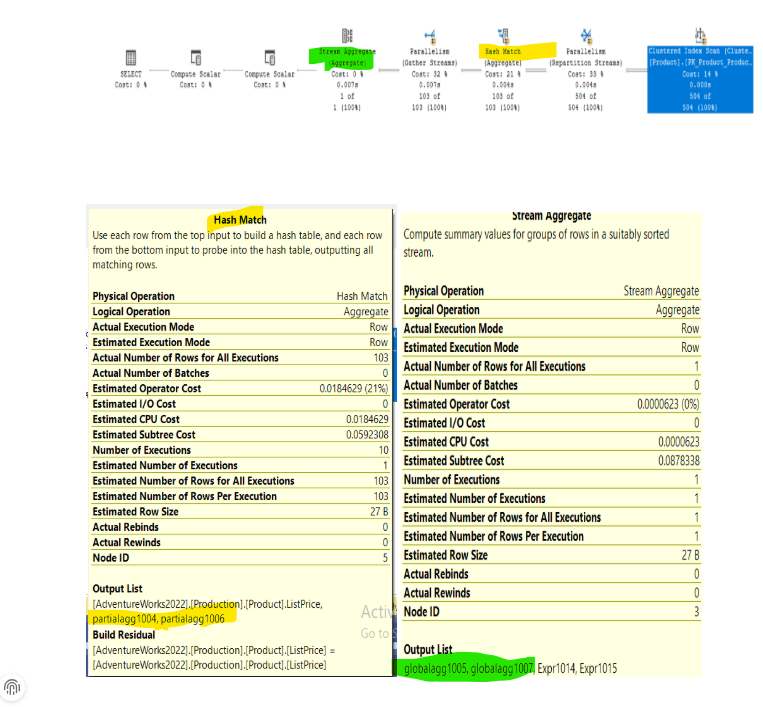
As you can see, it created a similar plan to what we saw in the rule, in the hash match it separated its aggregates to children, then, after the gather streams it combined them in one global stream, which was the global aggregate
Why did it discarded them? low row count makes the serial plan way more efficinet
Same for the hash
more on both in future blogs
But we can see in the traces, it considered both, even created physical and logical alternatives
With that, we finish today’s exploration of the plan