In the previous blogs, we introduced the two physical operators that SQL Server uses to aggregate values; today, we are going to explore the HAVING clause in that.

Filter operator with having

For example:

use AdventureWorks2022
go
select transactiontype,count(productid)product_count,sum(actualcost)as cost_total
from production.transactionHistoryArchive
group by transactiontype
having sum(actualcost)< 20
go

We get:

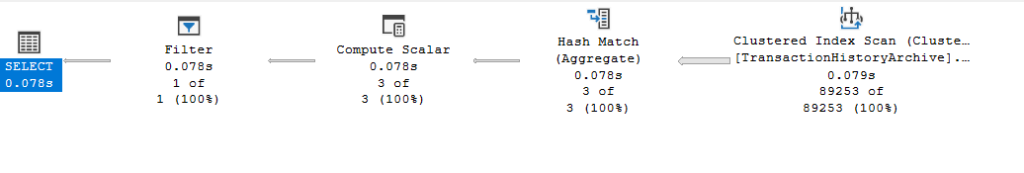
So:

• Scan the rows we need
• Create a hash key for 3 distinct values of transactiontype, the group by column
• while doing that, you know grouping by the hash aggregate, count and sum the values
• Then convert_implicit the count in the compute scalar
• And since you have no idea whether the having clause would match or not, since you don’t know the sum before actually aggregating it, filter by the clause we gave you

If we look at the filter operator:

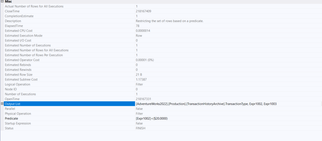
We can see it just filters by one of the previous calculated expressions in this case, the sum of the cost calculated in the hash aggregate

nothing much

But what if the optimizer knew the result before execution:

use AdventureWorks2022
go
select transactiontype,count(productid)product_count,sum(actualcost)as cost_total
from production.transactionHistoryArchive
group by transactiontype
having TransactionType = 'W'
go

We get:

No filter, since it knew the result beforehand, kind of like the where clause,

What rule did it apply to get this?

Traces with transformation rules

use adventureworks2022;

go
dbcc traceon(3604);
go

select transactiontype,count(productid)product_count,sum(actualcost)as cost_total
from production.transactionHistoryArchive
group by transactiontype
having TransactionType = 'W'

option (recompile, querytraceon 8605, querytraceon 8606, querytraceon 8607,
        querytraceon 8608, querytraceon 8621, querytraceon 3604,
        querytraceon 8620, querytraceon 8619, querytraceon 8615,querytraceon 8675, querytraceon 2372,querytraceon 2363)
go

We get:

*** Converted Tree: ***
    LogOp_Project QCOL: [AdventureWorks2022].[Production].[TransactionHistoryArchive].TransactionType COL: Expr1002  COL: Expr1003 
        LogOp_Select
            LogOp_GbAgg OUT(QCOL: [AdventureWorks2022].[Production].[TransactionHistoryArchive].TransactionType,COL: Expr1002 ,COL: Expr1003 ,) BY(QCOL: [AdventureWorks2022].[Production].[TransactionHistoryArchive].TransactionType,)
                LogOp_Project
                    LogOp_Get TBL: production.transactionHistoryArchive production.transactionHistoryArchive TableID=990626572 TableReferenceID=0 IsRow: COL: IsBaseRow1000 
                    AncOp_PrjList 
                AncOp_PrjList 
                    AncOp_PrjEl COL: Expr1002 
                        ScaOp_AggFunc stopCount Transformed
                            ScaOp_Identifier QCOL: [AdventureWorks2022].[Production].[TransactionHistoryArchive].ProductID
                    AncOp_PrjEl COL: Expr1003 
                        ScaOp_AggFunc stopSum Transformed
                            ScaOp_Identifier QCOL: [AdventureWorks2022].[Production].[TransactionHistoryArchive].ActualCost
            ScaOp_Comp x_cmpEq
                ScaOp_Identifier QCOL: [AdventureWorks2022].[Production].[TransactionHistoryArchive].TransactionType
                ScaOp_Const TI(nvarchar collate 872468488,Var,Trim,ML=2) XVAR(nvarchar,Owned,Value=Len,Data = (2,87))
        AncOp_PrjList 

So here we can see that the ScaOp_Comp x_cmpEq was evaluated after the aggregation, meaning it is not a child operator of LogOp_GbAgg OUT, meaning, when it first parsed the query without any re-writes, the query had the filter

But if we look at the simplified tree, way early on, before even cost-based optimization:

SelOnGbAgg rule predicate pushdown:

***** Rule applied: SelOnGbAgg - SEL GbAgg(x0,e0,e1) -> SEL GbAgg(SEL(x0,e0),e2)

    LogOp_GbAgg OUT(QCOL: [AdventureWorks2022].[Production].[TransactionHistoryArchive].TransactionType,COL: Expr1002 ,COL: Expr1003 ,)
      LogOp_Select
        LogOp_Get TBL: production.transactionHistoryArchive production.transactionHistoryArchive TableID=990626572 TableReferenceID=0 IsRow: COL: IsBaseRow1000 
        ScaOp_Comp x_cmpEq
          ScaOp_Identifier QCOL: [AdventureWorks2022].[Production].[TransactionHistoryArchive].TransactionType
          ScaOp_Const TI(nvarchar collate 872468488,Var,Trim,ML=2) XVAR(nvarchar,Owned,Value=Len,Data = (2,87))
      AncOp_PrjList 
        AncOp_PrjEl COL: Expr1002 
          ScaOp_AggFunc stopCount Transformed
            ScaOp_Identifier QCOL: [AdventureWorks2022].[Production].[TransactionHistoryArchive].ProductID
        AncOp_PrjEl COL: Expr1003 
          ScaOp_AggFunc stopSum Transformed
            ScaOp_Identifier QCOL: [AdventureWorks2022].[Production].[TransactionHistoryArchive].ActualCost

Now, as you can see here, it pushes down the having predicate as a filter of the aggregate, meaning like a where clause, since it knows that the values do not need to be known before aggregation, thus getting rid of the extra overhead

Now, we can precompute the sum if we like and get the same optimization, and the aggregate would be gone, so basically we would just have an index scan

Spool

If we do the following:

use AdventureWorks2022
go
select TransactionType, 
sum(actualcost) as total_cost, 
sum(productid) as total_product, 
sum(distinct(productid)) as something_pr,
sum(distinct(ActualCost)) as something_cost
from Production.TransactionHistoryArchive
where ActualCost < 20
group by TransactionType
go

This is a terrible query, but:

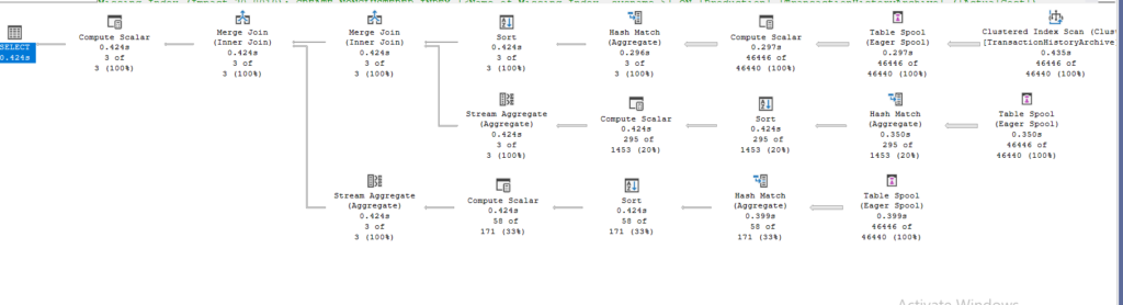
We get out our table spools, so what are they?

The optimizer realizes that we are asking for the scan multiple times

So instead of doing it over and over again, it does it once then it stores the data in memory, or if there is not enough of it spills, meaning it creates a worktable, and a worktable is a table created to store intermediate results for a query, and gives that to whoever needs it, in this case the other two aggregate functions.

The issue with that is the fact that it needs memory, lots of it

Secondly, it has to be inserted on a single thread, so no parallelism

The third concern, is that if we had a nested loop join, the scan instead of being stream lined like we see with the scan and a stream aggregate, has to be read from the beginning for each run, so we might have to scan it for every row if it was in the inner input, more on that later here

We have two types of spools in the sense of persistence, eager, which is a blocking operator, finishes scanning all the data, then stores it, and gives it to the other spools

The second type, lazy spool, which is the most common, processes row-by-row, so it is pipelined, so more efficient

We have the first type here.

Or it could be classified by the source of data, like a table spool here, or an index spool

Now, here since it scanned the clustered we got a table spool, but if we had an index, we could get an index spool, more on that later here

All the spools have the same nodeid = 6 in here, meaning they are the same operator, iterated over and over again

Properties of the spool:

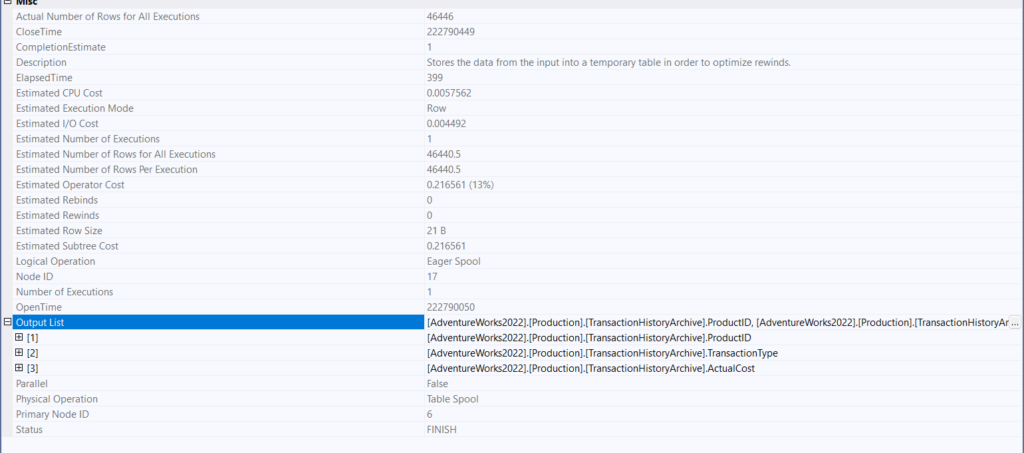
You can see, nothing too fancy, just a temporary table with the rows needed for the query

Now for the upper section of the query:

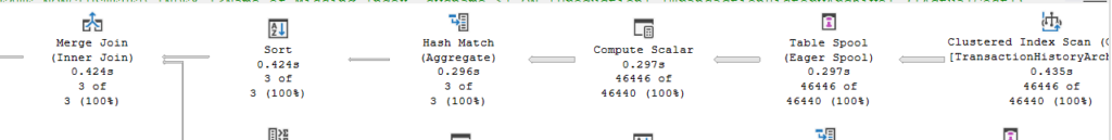
It scans, stores it in the spool, the compute scalar, and the sort are for the merge join

You need to sort to perform a merge join, more on that when we talk about join types in this series, and you need a join predicate, the compute scalar in each section servers that purpose, it ensures that our group by column, TransactionType, is the one in each section

In the properties of this hash aggregate:

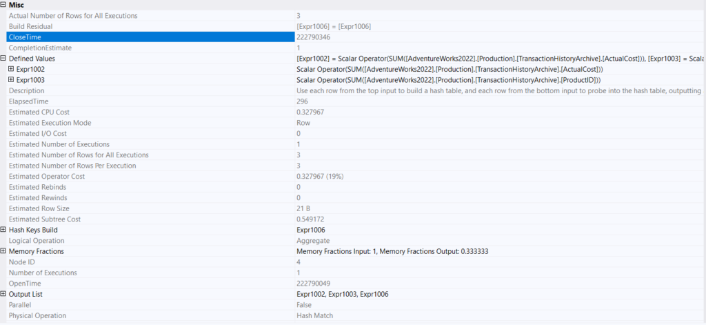
So you can see, here it counted the first two select aggregates, grouped by our TransactionType compute scalar output = expr1006, which is what made this hash key

So two regular old-fashioned counts cost one aggregate, and the sort was only there for the join, meaning distinct costs a lot, each of the other sections was for one of the distincts

If we look at the second section of the query:

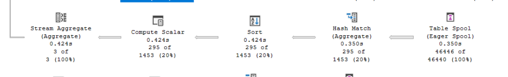
We got our table spool, which has the same node id, contains the same scan we collected before, that is the optimization

Hash aggregate:

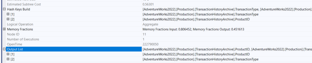
Now we know that the hash key needs to be unique for the algorithm to work, so hashkeys would guarantee that we have distinct values, so we don’t need the sort, but this sort here is for the merge join to work, not because we need the sort explicitly, same for the compute scalar, it guarrantes that, So we have the distinct values, but for both the stream aggregate and the merge join to work we need the sort, so it sorted and summed grouped by the TransactionType in the stream aggregate

The last section is the same as the second, but for the ActualCost column.

Aggregate with a spool and a nested loop join:

Now, if we do:

use adventureworks2022;
go

select 
    sp.businessentityid,
    sp.territoryid,
    soh.[total_of_subtotal:)]
from sales.salesperson as sp
cross apply (
    select sum(subtotal) as [total_of_subtotal:)]
    from sales.salesorderheader as soh
    where soh.territoryid = sp.territoryid
) as soh
;
go

We get:

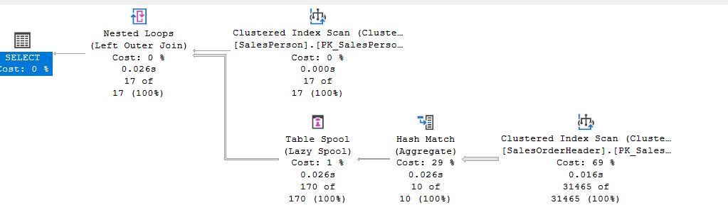
So for the cross apply’s hash aggregate:

• hash key build is on the territoryid = the filtering join condition
• and it sums and outputs them as an expression
• then the spool, which is lazy one, so it would take the rows one by one and compare them, but since the hash aggregate is a blocking operator, that did not happen here, anyway it gets the data, which is 10 rows, stores it, and runs it 10 against each of the 17 rows of the the sales.SaleOrderHeader, which is why we see the 170 row estimate

If we check the properties of the spool:

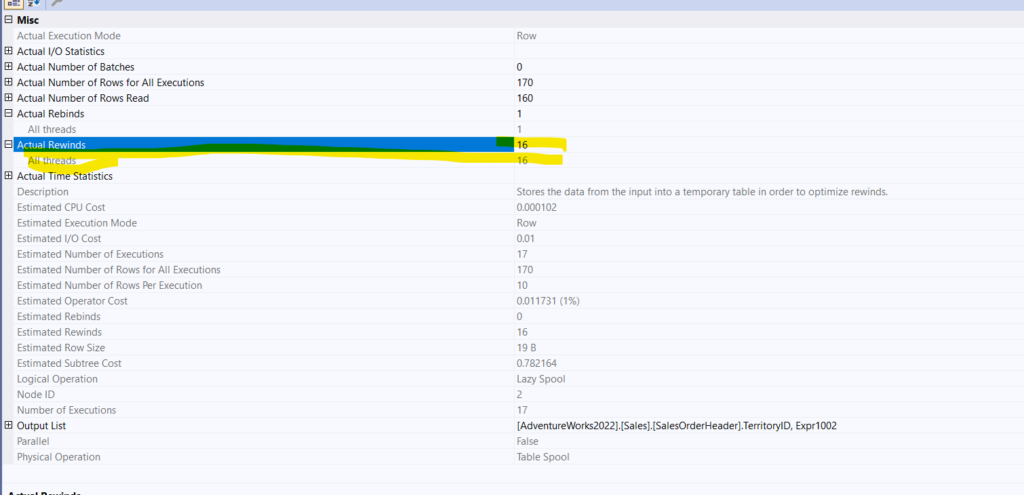
We see 16 rewinds, meaning after the first run, the lazy spool re-reads its data 16 times = 17

This is why spools are bad

And since you need to run the inner query per row from the outer input in the nested loop join(more on it in another blog), this would be highly inefficient

Now, if we seek in the inner query, we would get an index spool, but that did not happen here.

And we are done here, see you in the next one.