
In the last two parts of this series, we looked at scalar aggregates and how do they get computed, and we said that is the main difference is the group by clause, we don’t have there, but once we have it we start dealing with general purpose or vector aggregates that have a group by clause, the first one is a stream aggregate
Intro
Now for the data to be processed by a stream aggregate, it needs to be sorted based on the group by, now previously, since all the request, table, columns were treated as one group, since there is no group by, so we did not see a sort in the plan, because we don’t need it, but if we about to perform something with a group we have to see it
Also, we could have multiple columns in the group by, so how does the stream aggregate deal with them? Does it start with the first, then the second? Does it make a difference? What is the order of sorting in this situation?
It sorts regardless of order based on both columns
So if we had class and productline in the group by, it will use both, but it could be by class, productline, or the reverse
So far, so good
What about if we had an index that has the column sorted? then we don’t need the sort
What about if we had an explicit order by clause that specifies the sort order explicitly?
Then it has to stick to that while sorting, no reversing in there
Okay, how does the algorithm work?
Algorithm
The pseudocode provided by Craig Freedman and Conor Cunningham:
clear the current aggregate results
clear the current group by columns
for each input row
   begin
       if the input row does not match the current group by columns
          begin
             output the aggregate results
             clear the current aggregate results
             set the current group by columns to the input row
          end
      update the aggregate results with the input row
   end
Assume we have the following query:
use AdventureWorks2022
go
select class,avg(ListPrice)
from production.product
group by class
go
The plan would be:
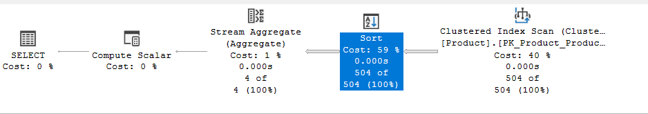
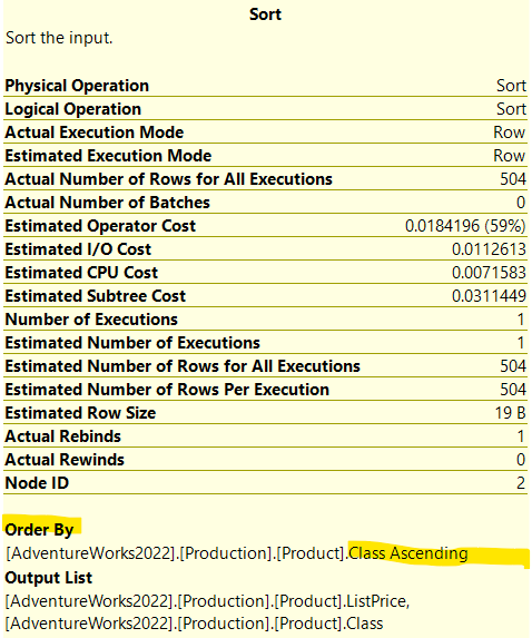
So here, after sorting the rows we requested from the table, which were class and listprice, the sort is based on class as an ascending key
which we know have 5 distinct values, groups, look for the data provided, and see if we have any aggregate results, aggregate group by columns, clear them, but since this is our first iteration there is nothing here, we don’t have to clean anything
For each input row, if the group by column is different,
Then, output the calculated results for the previous group column, which is nothing here
After you output them start from 0
and put the new input row’s group by column as the new group by column
Then add, update the results by adding the new value
then end
So now that we have the first class, see if the next sorted value matches the same row
if it does, add it.
and it keeps adding until it reaches the next group by columns
When it is there, it stops calculating, outputs the current results, and starts with the next group by class in the sorting order
And keep going until you finish
Then stop outputting
Graphical plan:
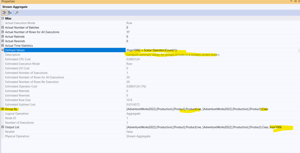
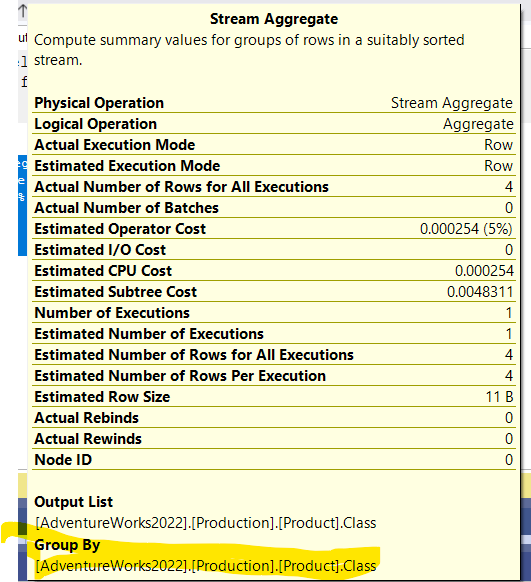
The stream aggregate properties:
- Defined values:
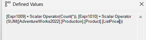
Like a regular AVG function, it just calculates the sum and count so it could put them in the next compute scalar, to give it to the select operator
But there is a new thing:
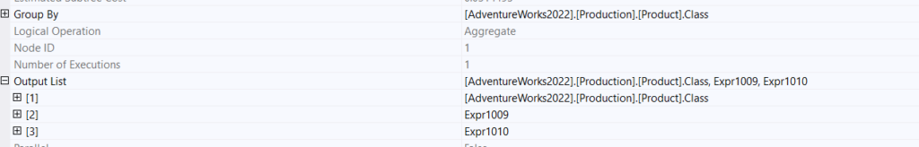
- Group By is the class, which is what we specified
- And outputs the group by column with sum and count, so the expressions could be processed by the compute scalar
- And after that, it outputs the last computed expression
- then select
And with that, this basic group by column is executed.
Multiple columns in the group by
Now we talked about the Order of columns where there is not an explicit order by clause, let’s see it in action:
use AdventureWorks2022
go
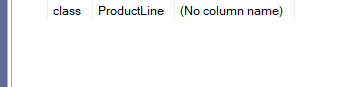
select class,ProductLine,count(*)
from production.product
group by class,ProductLine
go
We get:
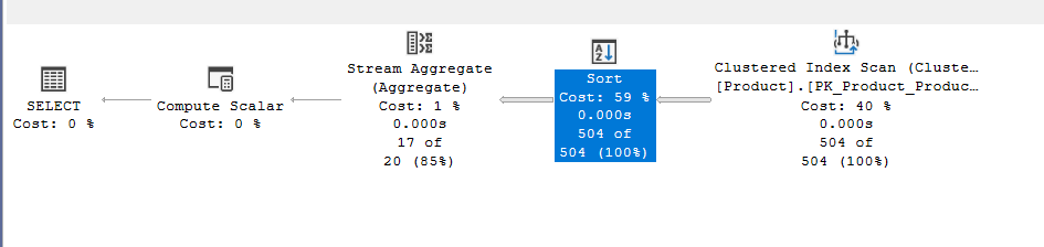
In the properties of the sort:
As you can see, it chose sorting by product line, then class, since we did not specify a specific order by, there is no importance of how the order by is sorted, it is just a function to feed to the stream aggregate
The only difference between this plan and the plan in the scalar( without a group by) is that this one has a sort order to help group the columns before aggregating them
Now, this order could have been reversed
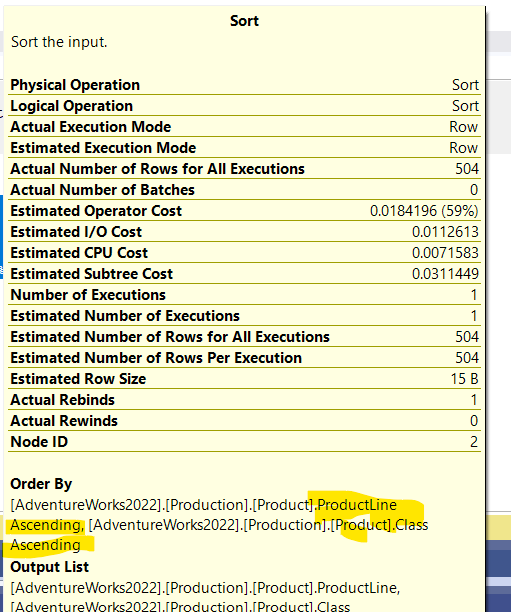
But if we explicitly specify an order like:
use AdventureWorks2022
go
select class,ProductLine,count(*)
from production.product
group by class,ProductLine
order by class, productline
go
We get:
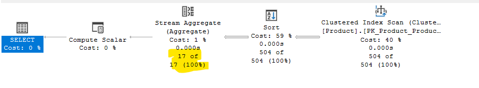
Back to the original query, after the sort we see the stream aggregate, now there is a cardinality estimation error, we will touch on how that happened in a bit
But if we look at the properties:
So here the computed expression is added to the output, since the count uses int, we would see the compute scalar after that, nothing fancy there.
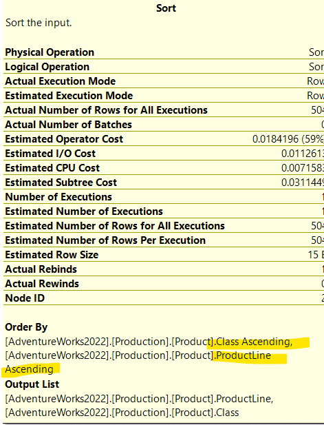
The textual plan:
|--Compute Scalar(DEFINE:([Expr1002]=CONVERT_IMPLICIT(int,[Expr1006],0)))
 |--Stream Aggregate(GROUP BY:([AdventureWorks2022].[Production].[Product].[ProductLine], [AdventureWorks2022].[Production].[Product].[Class]) DEFINE:([Expr1006]=Count(*)))
  |--Sort(ORDER BY:([AdventureWorks2022].[Production].[Product].[ProductLine] ASC, [AdventureWorks2022].[Production].[Product].[Class] ASC))
   |--Clustered Index Scan(OBJECT:([AdventureWorks2022].[Production].[Product].[PK_Product_ProductID]))
We can see the order by clause with productline first, then the class, since we did not use an explicit order by, all that stuff
Nothing to be noted in the XML:
<OptimizerStatsUsage>
   <StatisticsInfo Database="[AdventureWorks2022]" Schema="[Production]" Table="[Product]" Statistics="[AK_Product_ProductNumber]" ModificationCount="0" SamplingPercent="100" LastUpdate="2023-05-08T12:07:34.43" />
   <StatisticsInfo Database="[AdventureWorks2022]" Schema="[Production]" Table="[Product]" Statistics="[AK_Product_Name]" ModificationCount="0" SamplingPercent="100" LastUpdate="2023-05-08T12:07:34.43" />
   <StatisticsInfo Database="[AdventureWorks2022]" Schema="[Production]" Table="[Product]" Statistics="[AK_Product_rowguid]" ModificationCount="0" SamplingPercent="100" LastUpdate="2023-05-08T12:07:34.43" />
   <StatisticsInfo Database="[AdventureWorks2022]" Schema="[Production]" Table="[Product]" Statistics="[_WA_Sys_00000011_09A971A2]" ModificationCount="0" SamplingPercent="100" LastUpdate="2025-04-08T18:38:55.91" />
   <StatisticsInfo Database="[AdventureWorks2022]" Schema="[Production]" Table="[Product]" Statistics="[_WA_Sys_00000010_09A971A2]" ModificationCount="0" SamplingPercent="100" LastUpdate="2025-04-08T20:08:51.11" />
 </OptimizerStatsUsage>
We only mentioned these to use them in DBCC SHOW STATISTICS
Estimated row count in a multi-column group by clause
Now, for more on statistics and how to interpret them, you can check our blog HERE
The way that SQL Server estimates row count for group by with multiple columns is not documented, but Paul White made this formula, which gives us the same estimate as the query optimizer, now there he used extended events, trace flag 2363, now since we are not troubleshooting, and this is just for demonstration purposes, we are going to use that traceflag here:
use AdventureWorks2022
go
select class,ProductLine,count(*)
from production.product
group by class,ProductLine
option(querytraceon 3604,querytraceon 2363)
go
One of the computations for which was the calculation for our current plan, before it gets converted to a physical plan, was:
Begin distinct values computation

Input tree:

  LogOp_GbAgg OUT(QCOL: [AdventureWorks2022].[Production].[Product].Class,QCOL: [AdventureWorks2022].[Production].[Product].ProductLine,COL: Expr1002 ,) BY(QCOL: [AdventureWorks2022].[Production].[Product].Class,QCOL: [AdventureWorks2022].[Production].[Product].ProductLine,)

      CStCollBaseTable(ID=1, CARD=504 TBL: production.product)

      AncOp_PrjList

          AncOp_PrjEl COL: Expr1002

              ScaOp_AggFunc stopCount Transformed

                  ScaOp_Const TI(int,ML=4) XVAR(int,Not Owned,Value=0)

Plan for computation:

  CDVCPlanLeaf

      0 Multi-Column Stats, 2 Single-Column Stats, 0 Guesses

Loaded histogram for column QCOL: [AdventureWorks2022].[Production].[Product].ProductLine from stats with id 10

Loaded histogram for column QCOL: [AdventureWorks2022].[Production].[Product].Class from stats with id 9

Using ambient cardinality 504 to combine distinct counts:

  5

  4

Combined distinct count: 20

Result of computation: 20

Stats collection generated:

  CStCollGroupBy(ID=2, CARD=20)

      CStCollBaseTable(ID=1, CARD=504 TBL: production.product)

End distinct values computation

Begin distinct values computation
as you can see in Using ambient cardinality 504 to combine distinct counts: it used the two all_density for the producline and class auto-created stats, which we showed in the XML, were used and it gave us the ids and where there are, and it pointed out that it did not find any multicolumn stats, so to improve it we can do that or create an composite index on both
So when it did not find the multicolumn stats, it just used the auto-created multicolumn stats as it said, and the estimate was 20 ( CStCollGroupBy(ID=2, CARD=20))
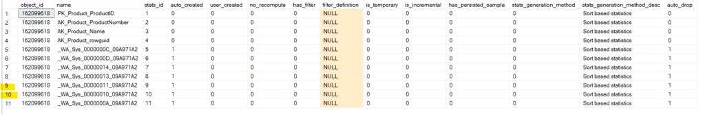
We can verify that by:
select*
from sys.stats
where object_id(N'production.product') = object_id
The output was:
And if we dbcc show_statistics like:
use AdventureWorks2022
go
DBCC SHOW_STATISTICS ('Production.Product', '_WA_Sys_00000010_09A971A2');
DBCC SHOW_STATISTICS ('Production.Product', '_WA_Sys_00000011_09A971A2');
go
You should use the auto-created at your environment, but ours was this ,and the all-density was:
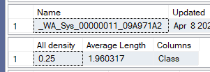
for class and for productline:
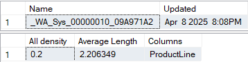
and all-density is 1/n where n = the number of distance values which was 4 and 5 respectively
So, how did it come to the number 20? Did it just multiply them(coincidence) like it did in the where clause in the old cardinality estimator(this is why this query is confusing)? I mean, we did not use the legacy or an older cardinality estimator XML:
No, it used a different formula that is in the above-mentioned blog by Paul White, we modified the initial parameters in the suggested formula like:
DECLARE
    @Card float = 504,
    @Distinct1 float = 5,
    @Distinct2 float = 4;
------ for the other stuff check out Mr.Paul White's blog
And the result was like:
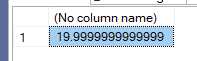
Which is the 20 we saw, but since there are some combinations that in group by that did not have any rows in it, like:
use AdventureWorks2022
go
select class,ProductLine,count(*)
from production.product
where Class = 'H' and ProductLine = 'S'
group by class,ProductLine
order by Class,Productline
option(querytraceon 3604,querytraceon 2363)
go
A difference between scalar aggregate and regular vector aggregates where there are no rows to output
Now we quoted Craig Freedman before, where he was talking about scalar aggregates:
Note that a scalar stream aggregate is one of the only examples (maybe the only example – I can’t think of any others right now) of a non-leaf operator that can produce an output row even with an empty input set.
But that is not the case here; the output was:
no null, no 0
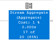
Back to the previous conversation, why the 20 was actually 17, some combinations like class = h and productline = s are empty, do not have any rows, which was not accounted for in the estimate, since we don’t have multicolumn statistics
So it had 17 full combinations, which is why the CE was off a bit :
Now, if we create multicolumn stats like:
create statistics test_multi
on production.product (class, productline);
and query like:
use AdventureWorks2022
go
select class,ProductLine,count(*)
from production.product
group by class,ProductLine
order by Class,Productline
option(recompile ,querytraceon 3604,querytraceon 2363)
go
We get:
And if we check the trace output:
Begin distinct values computation

Input tree:

  LogOp_GbAgg OUT(QCOL: [AdventureWorks2022].[Production].[Product].Class,QCOL: [AdventureWorks2022].[Production].[Product].ProductLine,COL: Expr1002 ,) BY(QCOL: [AdventureWorks2022].[Production].[Product].Class,QCOL: [AdventureWorks2022].[Production].[Product].ProductLine,)

      CStCollBaseTable(ID=1, CARD=504 TBL: production.product)

      AncOp_PrjList

          AncOp_PrjEl COL: Expr1002

              ScaOp_AggFunc stopCount Transformed

                  ScaOp_Const TI(int,ML=4) XVAR(int,Not Owned,Value=0)

Plan for computation:

  CDVCPlanLeaf

      1 Multi-Column Stats, 0 Single-Column Stats, 0 Guesses

Using ambient cardinality 504 to combine distinct counts:

  17

Combined distinct count: 17

Result of computation: 17

Stats collection generated:

  CStCollGroupBy(ID=2, CARD=17)

      CStCollBaseTable(ID=1, CARD=504 TBL: production.product)

End distinct values computation
You can see, it used the multi-column stats
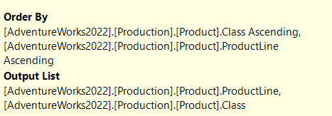
Using an index to get rid of the sort:
Now, for the stream aggregate to work efficiently we saw that it needed a sort that has an implicit or an explicit order by, but if the index Has them sorted, we don’t need that operator:
create nonclustered index ix_class_producline_product on production.product(class,productline)
execute:
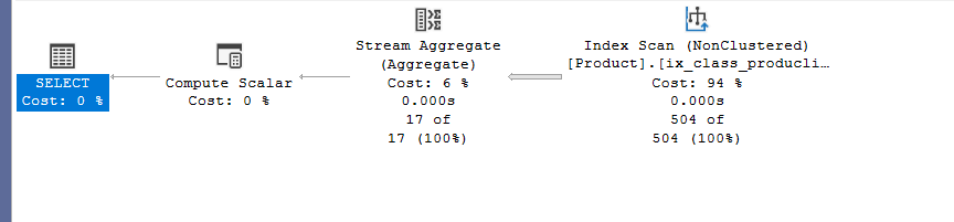
No sort, since we have the order in the index.
Using the index to make efficient distincts
Now, DISTINCTS need a sort no matter what the query is, for example:
select distinct(class) from production.product
We get:
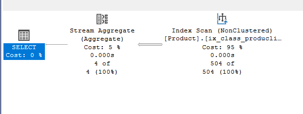
Now,why would it have a stream aggregate? Distinct is a group by the whole column as a group
Even if we rewrite it like this:
select distinct(class) from production.product group by class
We get the same plan and in the properties:
In the first query, with no group by
Distinct aggregates,using stream aggregate instead of distinct sort
Now, let’s drop the index we just created
drop index ix_class_producline_product on production.product
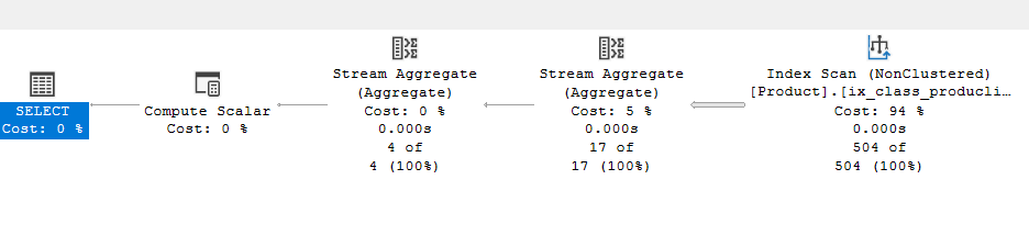
Now, if we run this:
select class, count(distinct(productline))
from production.product
group by class
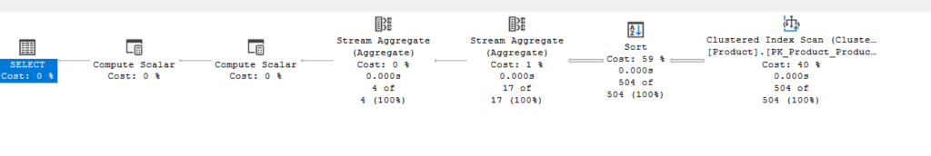
We get:
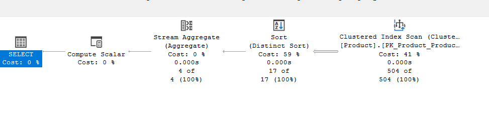
The distinct sort properties:
So, it had to sort them on both before aggregating, since it had to know the groups created by class, and it wants to know the distinct of the productline, so we get the sort distinct for both
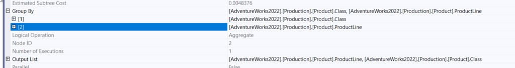
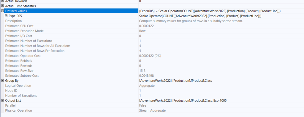
In the stream aggregate:
So, it grouped the distinct results of productline by class, to know how many there are in each group
The expression is for the count before conversion with a compute scalar to an int
Now, if we recreate the index like:
create nonclustered index ix_class_producline_product on production.product(class,productline)
and re-execute:
use AdventureWorks2022
go

select class, count(distinct(productline))
from production.product
group by class
go
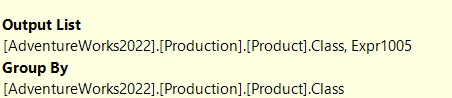
The first stream aggregate:
So, as you can see here, it did not count anything, it just replaced the sort, since the sort is provided with our index, and put the values of each column next to each other
In the second stream aggregate:
We see that it grouped the productline by each class, then counted them, and output the expression before the conversion with the compute scalar
That is how we replace the distinct sort.
Now, drop the index before going:
drop index ix_class_producline_product on production.product
Multiple regular and DISTINCT aggregates
Now, if we do the following:
select class, count(*), count(distinct(productline))
from production.product
group by class
We get:
Here we see a different implementation of GenLGAgg. in the previous blog, we saw how it could generate parallel alternative plans, but here there is something different, more on it in the next blog.