Hi everyone,

in the previous blogs, we said that the query optimizer has a cost-based model while generating the plans, and based on that the optimizer might choose different physical operators.

to do that it needs to know how many rows will be returned by the query = cardinality estimation

and to make that estimation it needs a basic understanding of the data,

and to do that you need statistics, the more accurate they are, the better the estimates, and the better the execution plan we get.

today we are going to introduce these concepts.

Note: some of DMVs, DMFs, or trace flags we use in our blogs either are undocumented so Microsoft would not be responsible for any use of it if it corrupts data or introduce performance issues. and some of it introduces too much overhead. so you should not use the first unless it is a testing enviroment, and you should not use the second one in a production enviroment without the proper testing.

Statistics:

so the engine creates statistics to estimate:

• the number of rows returned by each operator = cardinality estimation = rows returned by a join
• selectivity: how many rows satisfy a specific condition = filter = where clause or a join filter = ON clause in a join

How does the engine create stats:

3 ways:

• auto when it’s on( it is by default, the command is: AUTO_CREATE_STATISTICS)
• when we create an index
• using CREATE STATISTICS explicitly

it could be created on multi-columns or one column

Auto-created stats are only on one column

we have 3 statistical objects:

• histograms(only on the first column)
• string statistics( only for strings)(only on the first column)
• the density information: how selective is the column

filtered indexes or statistics which is statistics explicitly created with a where clause does not get created automatically we have to create it.

once they are created they can be updated automatically.

statistics can get outdated = new data has been inserted and the current stats does not represent the current data distribution

now the default, which is auto-updating will generate better plans since the optimizer relies on them,

but every time we run a query before and after, we have to recompile it again, and we have to wait for the stats to get created, which could cause delays, on some systems this can be modulated to updates during downtime making the process more efficient.

the size of the sample of the database that the SQL server gets depends on the table and the version,

the minimum is 8mbs or lower for smaller tables,

however, we can manually assign the specific percentage that we want to sample explicitly

for example, we could use FULLSCAN

this could benefit us, especially in large tables that don't have random distribution

for example

if SQL server opts to use only 50 percent of the table, it will assume that the rest of it will match the current distribution

which could skew the estimated row counts depending on how far the 50 percent is far from the model.

we could make the query faster by choosing AUTO_UPDATE_STATISTICS_ASYNC making the process non-blocking,

this would make the query capable of executing without waiting for the stats, at the expense of having outdated ones

when does the stats get outdated?

it tracks column modification counters or ColModctr

so every 500 modifications plus 20% of table size the stats gets updated

this was the old model which had to use the 20 percent threshold

in SQL server 2008 traceflag 2371 was introduced, which fixes the problem by introducing a dynamic threshold

tables with row amount lower than 25 000 rows will still use the 20 percent rule, but once it grows the ColModctr will get triggered dynamically at lower percentages

this traceflag is on by default in SQL server 2016 and above

let’s follow an example: if we have a permanent table with rowcount lower than 500

the stats will get updated every 500 row adds

if a table has more than 500

like let’s 2000

and the engine needs to calculate the threshold

it has 2 formulas

the first is 500 +(0.2 n) n in here number of rows in the table

so in 500 + 400= 900rows added would trigger that

or SQRT(1000*n) = the square root of 1000 *2000 = 1414…..

so the first one is the lower so it gets picked by the engine

in our case it was the first formula

now let’s assume that our tables rows are 25 000

the first would bee 500 +(25 000 * 2/10) = 5500

and the second one would be the square root of ( 1000 * 25 * 1000) = 1000* 5 = 5000

so now either formula could work

now let’s assume it is a million

so the first one would be 500 + (1 000 000 * 2 /10) = 200 500

the second one would be 31 thousand something

now the second one obviously would be lower

and hence the trace flag and the new way of updating stats is better than the first at large tables since it recognizes changes way earlier and updates the stats making the query estimates more accurate

now temporary table thresholds might be lower at first,

but in larger numbers both use the same formulas

Looking at the stats objects

one of the DMVs that could be used to inspect the stats is

sys.stats

for example:

USE AdventureWorks2022 
SELECT*
FROM sys.stats

we can see the following

the first one is the object_id = it is only unique in the database

the name

stats_id= equals the index_id if it was created with the on index otherwise each one is only unique to the index it is created on

auto or user_created= is it created by auto_update_statistics or is it explicit from the user

no_recompute = should we update the stats or should we create it once and let the user update it on his own

has_filter= is it created on where clause or on a filtered index, the filter definition would show if it had filter

is_temporary: something related to high availability groups,(the stats created on read only secondary )

is_incremental: created on partitions, is this stats has the option of being created on partitions enabled

has_persisted_sample: did you specify the sampling rate, did you say you want half or 20 percent of the table to be scanned when creating stats or did you just let it go dynamically through the formula we described

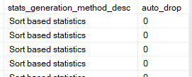
auto_drop= Would this user-created stats block schema modification statements or not

if no then 1 since this is what this option does

if yes then 0

only relevant for the stats created manually

another relevant DMF is

sys.dm_db_stats_properties, dynamic management function

we need to supply object_id and stats_id from the first DMV sys.stats

for example:

SELECT*
FROM sys.dm_db_stats_properties(OBJECT_ID('Sales.SalesReason'),1)

and the output would be like:

so the first two columns are the values we supplied

then we have the last time it was updated

how many rows in the table

how many rows were sampled from the table

the steps in the histogram (more on it later)

unfiltered rows= how many rows were not included in a where or an on clause in a join

modification_counter= how many rows were added/modified after the last stats update

persisted_sample_percent=what sampling percentage did the user specify

this DMF are only for non-incremental stats, meaning the one that does not have partition based stats

if we want to see incremental stats we should use: sys.dm_db_incremental_stats_properties.(more on it later)

another important DMF

sys.dm_db_stats_histogram, dynamic management function

we can see the histogram information here

for example;

SELECT*
FROM sys.dm_db_stats_histogram(OBJECT_ID('Sales.SalesReason'),1)

the output would be like:

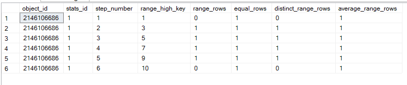
the histogram contains about each step in the data, meaning each range of data

fore example here in the first range = step

we can see that:

range_high_key = 1 which means the highest value here is 1

range_rows= 0 meaning the values other than range_high_key in the range between the last range nad the range_high_key value other than 1 is 0 so there are no values other than 1 in this range(more on it in a minute)

equal_rows: how many rows are equals 1, meaning the highest value in the range, meaning the range_high_key.

distinct_range_rows: how many rows in excluding the range_high_key value has distinct values so there are no duplicates in it

average_range_rows: number of rows returned per distinct value beside the highest value(the range_high_key), calculated as range_rows/distinct_range_rows but here since it is zero it just included 1

now let’s do the next step

step is the second, so it is the second range

the range_high_key= 3 and the last range_high_key =1 so the values from 1 to 3 excluding 1

range_rows = how many rows between 1 and 3 excluding both so there is one value here

equal_rows= there is one 3 here, one value equaling the range_high_key

distinct_range_rows= how many distinct values between the two range_high_key here 1

average_range_rows= how many rows would be returned per distinct value other than 3 here it is 1 which could be calculated like = average_rows/distinct_range_rows=1/1

so it is 2

same goes for steps 3, 4, and 5

now if we select the object itself PK_SalesReason_SalesReasonID like:

select SalesReasonID
from Sales.SalesReason

we can see

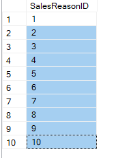
as the histogram said

so between 1 and 3 we had one distinct value that is two that has no duplicates and when selected would probably return 1 row

DBCC SHOW_STATISTICS(OBJECT_ID,STATS_ID)

It shows the same information, the header information like sys.dm_db_stats_properties(), the histogram information like sys.dm_db_stats_histogram(), and extra deprecated density information that is not being used by the optimizer anymore

for example

USE AdventureWorks2022 
DBCC SHOW_STATISTICS('Sales.SalesReason',PK_SalesReason_SalesReasonID)

the output would be like:

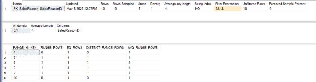
so first we have the header that contains:

the name, the last time the data was updated, how many rows does the table has, how many rows were sampled, the steps in the histogram, the average key length, meaning the single column in bytes, whether it is a string or not, is it a filtered stats or an index, how much of it was unfiltered and at which rate it was sampled 0 means the default

we can also Density

which is : means the density of values sampled except the range_high_key values it is deprecated and only there for backward compatibilty

then we move on to the density information:

in our example, we had 10 values so N is 10

and all density for this column is 1/N so 0,1 as you can see

the average length in bytes is 4

and the column is SalesReasonID

then we see the same output of

sys.dm_db_histogram_stats.

let’s look at a more complicated example

first, let’s create some stats:

create statistics order_saor_id_stats on Sales.SalesOrderHeader(SalesOrderID,OrderDate)

now if we:

dbcc show_statistics ('Sales.SalesOrderHeader',order_saor_id_stats)

the output would be like:

MultiColumn Statistics:

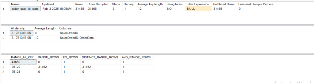
so we have the regular stuff at the top

then at the bottom we can see that the stats are calculated only for the leftmost columns hence the step values 43659 not a a date

now we can see all the steps in 3 steps

so even though SQL serve can go up to 200 steps we only see the 3

now if we create:

create statistics orderdate_stats on Sales.SalesOrderHeader(OrderDate)

and:

DBCC SHOW_STATISTICS('Sales.SalesOrderHeader',orderdate_stats)

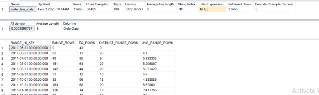
Now we have Col stats that is created on order date

, let’s try another method

now lets drop the stats above:

drop statistics  sales.salesorderheader.order_saor_id_stats
drop statistics  sales.salesorderheader.orderdate_stats

now let’s query the following:

SELECT*
FROM Sales.SalesOrderHeader
WHERE OrderDate = '2011-05-31 00:00:00.000'

we can in the following see:

DBCC SHOW_STATISTICS ( 'Sales.SalesOrderHeader', EngineGeneratedValue)<br>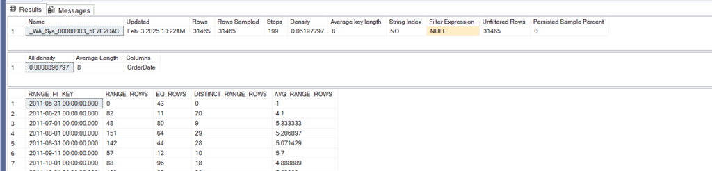

now the stats got auto-created since we used the column in the where clause

it is the same as before 199 steps and all

all density = selectivity so the lower it is the lower the value

The density vector: (all density)

for example

DBCC SHOW_STATISTICS('Sales.SalesOrderHeader',IX_SalesOrderHeader_SalesPersonID)

we can see the following

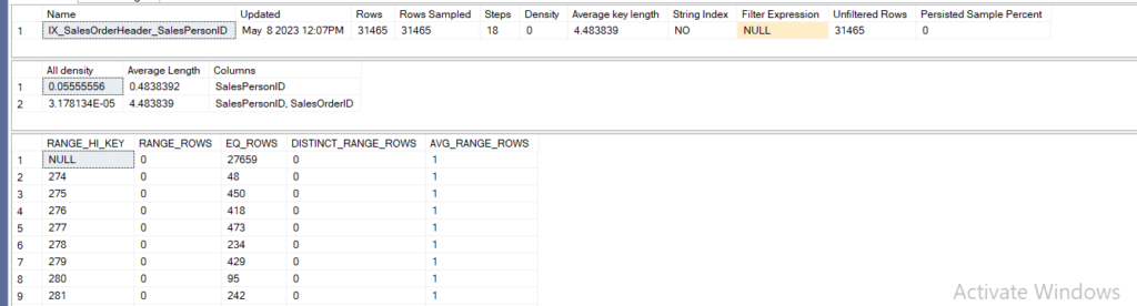
so it has 18 steps

all the rows were sampled

the first all-density or density vector was 0.05555556 which is:

since there was about 27659 nulls we have to exclude them from the calculation

and since the stats are built on leftmost indexes only

and since not all the salesperson id is distinct, as we can conclude from the histogram

for example

274 has range_rows and it has 48 equal_rows so it has 48 duplicates

we could prove that by

select distinct(SalesPersonID), COUNT(*)
FROM Sales.SalesOrderHeader
group by SalesPersonID

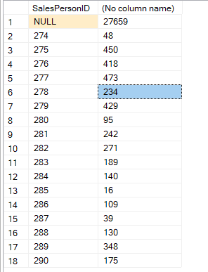
we see only 18 distinct values which means

1/n = 1/18 = 0.05555556

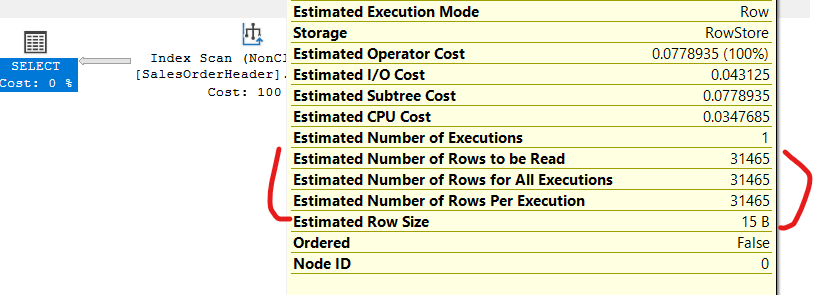
now if we look into the combined stats of the second one

sales order id is not null and there is one for each order in salesorderheader

so 1/n = 1/31465= 3.178134435086604e-5

as you can see the selectivity in this index for this columns combined is way higher

how would that affect us?

it would help the optimizer estimate how many rows will be returned by the group by

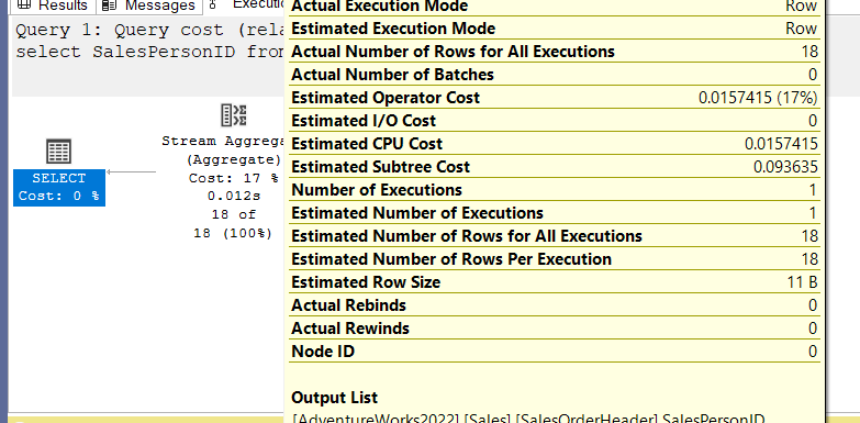
for example:

select SalesPersonID, SalesOrderID
from Sales.SalesOrderHeader 
group by SalesPersonID,SalesOrderID

as you can see it estimated the exact amount

and here the optimizer chose not to include the stream aggregate since the values are already sorted in the index itself

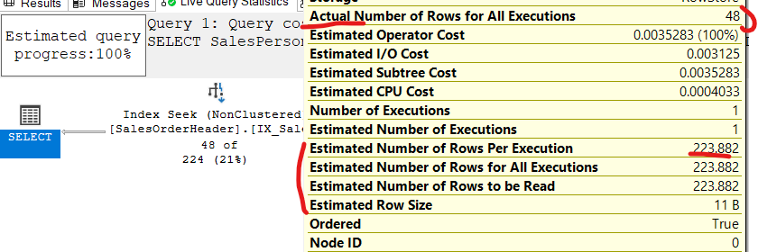
now if we look into the other one SalesPersonID

select SalesPersonID
from Sales.SalesOrderHeader
group by SalesPersonID

we can see:

so it estimated 18 will be returned the complementary value to 0.05555556 which was 18

,meaning the complementary to the all density value

now if we use local variables like:

DECLARE @SalesPersonID int 
SET @SalesPersonID = 274
SELECT SalesPersonID
FROM Sales.SalesOrderHeader 
WHERE SalesPersonID = @SalesPersonID

now as you can see there is a difference between the actual rows seeked which was 48

and what the engine estimated

the main reason here is the variable

they don’t have stats on them

so @SalesPersonID =what is going on? in SQL server terms

so it tries to guess

here it used the all_density information provided above

which was 0.05555556 multiplied by all the rows excluding the nulls which was 3806

211.4445

so here it optimized for nulls, as it had them as a histogram step which is a feature of the new cardinality estimator(more on it later)

now here since we used an equality operator it guessed through the density

if we used an inequality operator like:

DECLARE @SalesPersonID int 
SET @SalesPersonID = 274
SELECT SalesPersonID
FROM Sales.SalesOrderHeader 
WHERE SalesPersonID > @SalesPersonID

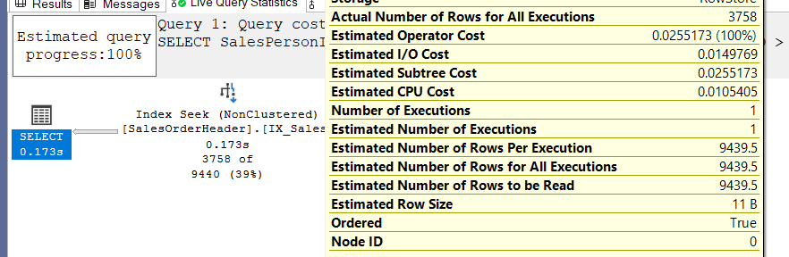
so why there is a difference and not the one we expected?

like we said before here it can’t use the guess

so it uses 30 percent rule of 31465 which is 9439.5

so instead of using that we should use either literals like we used before

or parameters like:

CREATE PROCEDURE GetSalesPersonID
@SalesPersonID int
AS 
BEGIN 
SELECT SalesPersonID
FROM Sales.SalesOrderHeader
WHERE SalesPersonID = @SalesPersonID
END 

Now let’s execute it

EXECUTE GetSalesPersonID 274

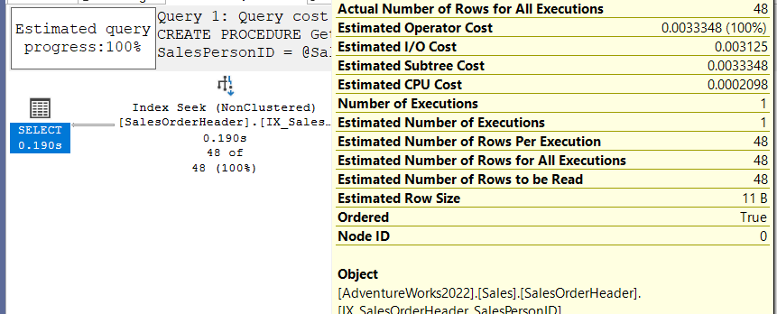
as you can see it used density information like you would not believe

How does the optimizer use the values in the histogram

now here I am going to use StackOverflow database you can reach from here

so let’s do our thing with dbo.Badges

dbcc show_statistics('dbo.Badges',IX_UserId)

and you can see the following

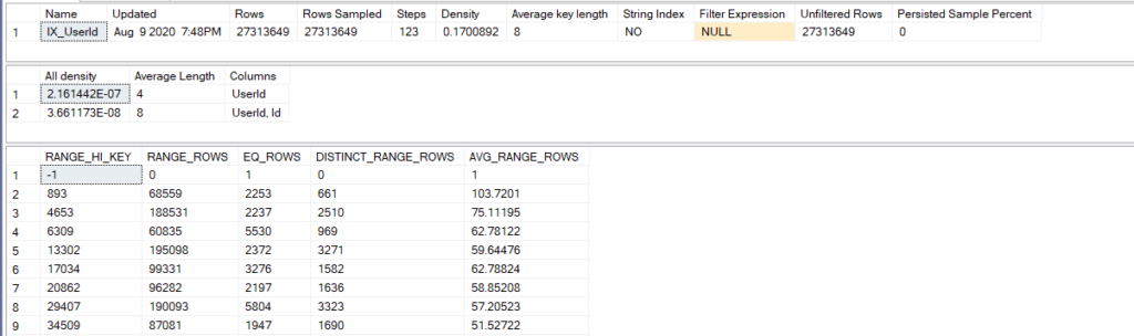
so as you can see

in the second range_high_key 893 we can see 661 distinct_range_rows

so even in the first range, we can see more than 200 distinct values

but the engine records only 200 unique and then estimates for the others

the algorithm used in there is called the maxdiff

it records the most frequent unique values in the distribution

so we see them

how does the engine use that:

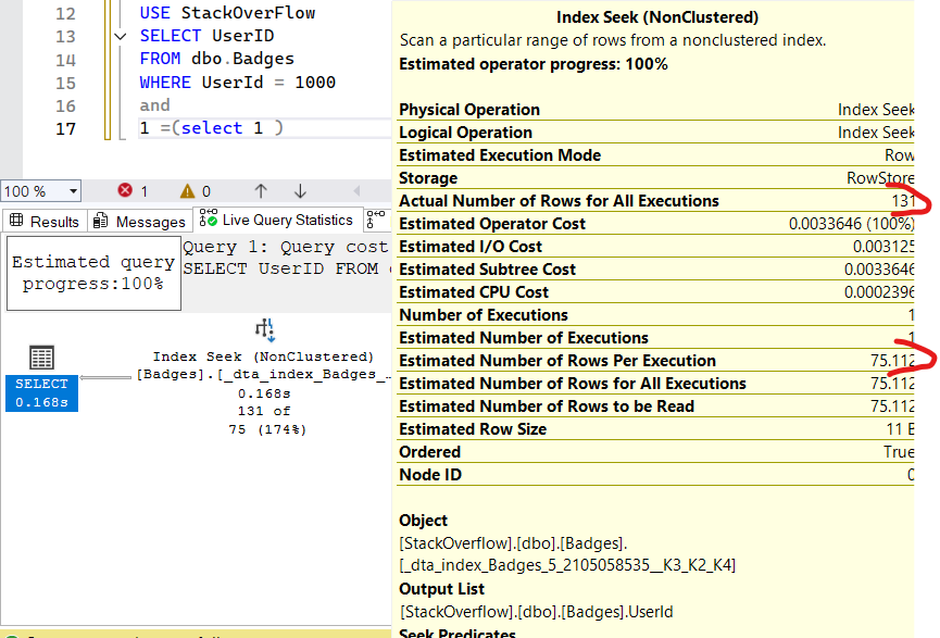
like we saw before if we specify a range_hi_key value in the where clause like:

USE StackOverFlow 
SELECT UserID
FROM dbo.Badges 
WHERE UserId = 893 

the plan estimates would be like:

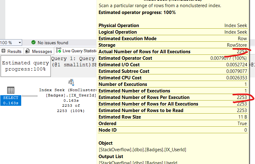
which is exactly the same as eq_rows

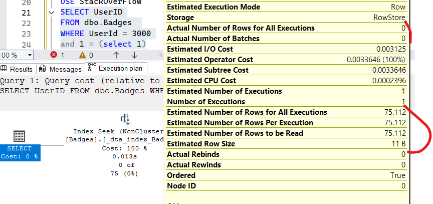
but if we do the same for a value in the range_rows like

USE StackOverFlow 
SELECT UserID
FROM dbo.Badges 
WHERE UserId = 1000
and 1 = (select 1) -- erik darling

we can see that the estimates are the same as the third range between 893 and 4653

so it returns the same value for everything in between let’s try another example:

USE StackOverFlow 
SELECT UserID
FROM dbo.Badges 
WHERE UserId = 3000
and 1 = (select 1)

now let’s use and inequality operator:

 USE StackOverFlow 
SELECT UserID
FROM dbo.Badges 
WHERE UserId > -1 and  UserId <6309
and 1 = (select 1)

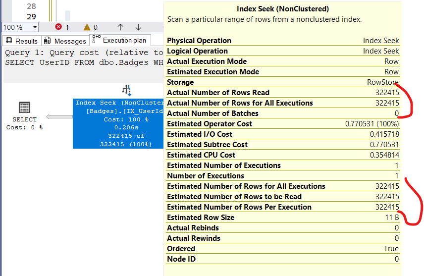
now here it adds the following:

• each range_hi_key values except the inequality operators
  • 2253
  • 2237
• each range_rows count
  • 68559
  • 188531
  • 60835

and you would get 322415 the same as the estimate

or we could use multiple predicates but this depends on the cardinality estimator:

Cardinality Estimator

this is the component of the query processer that estimates how many rows will be returned.

as we saw before it helps with query execution

it is based on statistics

which is inherently an inexact science that bypasses the random values and focuses on trends

it has several assumptions that the documentation presents:

• independence: the data between columns is not correlated, unless specified.
• uniformity: distinct values are evenly spaced( this is how it estimates the range values when used as prediactes as we showed before) and they all have the same frequency( even though our 3000 example had non)
• Containment(simple): users don’t query for nulls, or query for data that exists, or there is no nulls in the data
• inclusion: if we have a predicate that includes a constant like WHERE ProdcutId = 3 SQL server assumes that the 3 exists

now with the new one:

• independence is not here anymore we have correlation: the data is not necessarily independent now they can be really correlated
• Base Containment: now it does not assume that users does not query nulls.

now we will try both you should not change them unless you know what your doing

before 2014 trace flags as improvements had to be enabled through them now they are just on by default

before that trace flag 2312 to enable new cardinality estimator

and 9481 is used to disable it

both are documented

now we are going to explain the differences between both

so let’s do that

ALTER DATABASE stackoverflow
SET Compatibility_LEVEL = 100

Now its the 2008’s cardinality estimator(docs)

now let’s get back to our dbo.badges

so we know the UserID stats for example:

select*
from dbo.badges 
where userid = 1000

it estimated the rows from the histogram

now let’s see another column we could filter by

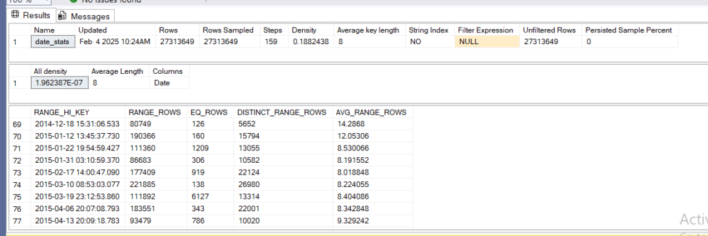
let’s create stats on date

CREATE STATISTICS date_stats ON dbo.Badges(date) WITH FULLSCAN;

now let’s see its stats and histogram

DBCC SHOW_STATISTICS('dbo.badges',date_stats)

now let’s do a select:

select*
from dbo.badges 
where date = '2015-02-03 10:49:40.360'

the estimates would be like

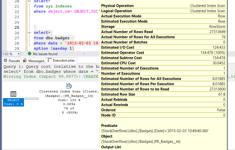
so it looked up the histogram then gave us the estimate

here we dropped an index before the execution so it had to scan the clustered to get it

now if we filter by both like:

SELECT*
FROM dbo.Badges 
WHERE date = '2015-02-03 10:49:40.360'
and 
UserId = 199700

we would get this estimate:

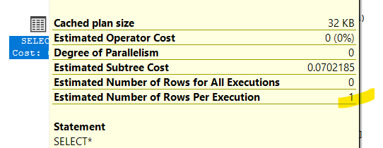
so how did it get this 1 :

• it goes to the first histogram for userid 199700 it looks up the selectivity which in our case was 21.30688/27313649
• then it goes to the second histogram does the same 8.018848/27313649
• then it multplies them by the number of rows 27313649
• which could be rounded up to 1

now in the new cardinality estimator:

ALTER DATABASE StackOverflow SET COMPATIBILITY_LEVEL = 160

if we run the same query again

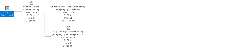
we would get the same estimate but the formula here is

the most selective predicate's selectivity which is 8.018848/27313649

multiplied by the square root of the second 8.018848/27313649

since both are rounded up to one it does not make much of a difference since both are very selective

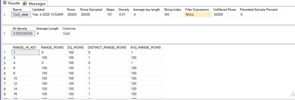
another example

the setup would be with two columns each has 300 distinct values and 100 for each

CREATE TABLE Number (
    Col1 INT,
    Col2 INT
);

WITH Numbers AS (
    SELECT TOP (300) ROW_NUMBER() OVER (ORDER BY (SELECT NULL)) AS num
    FROM sys.all_columns
)
INSERT INTO Number (Col1, Col2)
SELECT num, num
FROM Numbers
CROSS JOIN (
    SELECT TOP (100) ROW_NUMBER() OVER (ORDER BY (SELECT NULL)) AS r
    FROM sys.all_columns a
    CROSS JOIN sys.all_columns b
) Replicate;

now let’s create stats on both

create statistics Col1_stats on dbo.Number(Col1)
create statistics Col2_stats on dbo.Number(Col2)

let’s query the stats

DBCC SHOW_STATISTICS('dbo.number',Col1_stats)
DBCC SHOW_STATISTICS('dbo.number',Col2_stats)

we would get

so let’s run our select and alter the comapatibilty level

ALTER DATABASE StackOverflow SET COMPATIBILITY_LEVEL = 100

select*
from number
where col1 = 11
and col2 = 11

we get the following

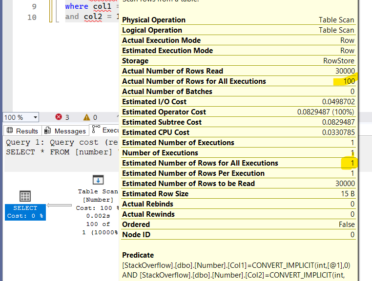
what happened here is the same:

• first row selectivity 100/30000
• second row selectivity 100/ 30000
• multiply by 30000
• 0.3333333333333333
• then it rounds it up to one and we get the estimate

now let’s alter again and select

ALTER DATABASE StackOverflow SET COMPATIBILITY_LEVEL = 160

select*
from number
where col1 = 11
and col2 = 11

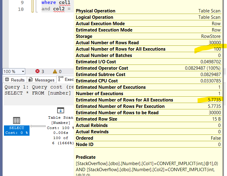
so here we get a better estimate:

• the most selective predicate’s selectivity(does not matter here ) 100/ 30000
• the square root of the second 100/30000
• multiplied by 30 000

and we would get the same estimate 5.7735

so first one assumes that the data is not correlated and produces the estimate on that assumption

the second one says they might be correlated

now let’s use the or in predicates:

ALTER DATABASE StackOverflow SET COMPATIBILITY_LEVEL = 100
select*
from number
where col1 = 11
or col2 = 11

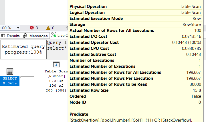
how did it come to this paritcular value:

as you can see we calculated the number of rows returned to the and in predicates as 0.3333333333333333

so it took it’s reciprocal by excluding the and predicate’s estimate from the total rows that could be returned by both predicates which was 200-0.3333333333333333= the value you see

and that is it.

for the or predicate in the new cardinality estimator, we can check paul white

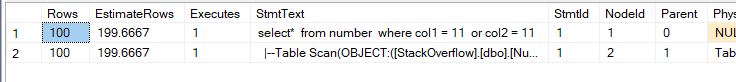
another easier way to show the actual vs the estimated rows

like we showed before in the previous blog

we can use set statistics profile on like:

use StackOverflow
ALTER DATABASE StackOverflow SET COMPATIBILITY_LEVEL = 100
go
set statistics profile on
go
select*
from number
where col1 = 11
or col2 = 11
go
set statistics profile off 

Statistics On Computed Columns

scalar expression generally can’t use stats

for example:

select*
from Sales.SalesOrderHeader
where Status*SalesOrderID > 50000 

the estimate was like:

the estimate was like 9440 which was 1/3 of the total rows of the table

which means in this case it just did not use any stats

it just guessed that 1/3 of the table would be returned

status is always 5

so it will always be true

so it should get all the rows of the table as estimate

but since it can’t do that

it just guessed 1/3

now if we create a computed column like :

ALTER TABLE Sales.SalesOrderHeader
ADD NEW_COMPUTE AS Status*SalesOrderID;

Now we have no stats on it unless we query it so:

select*
from Sales.SalesOrderHeader
WHERE NEW_COMPUTE>50000

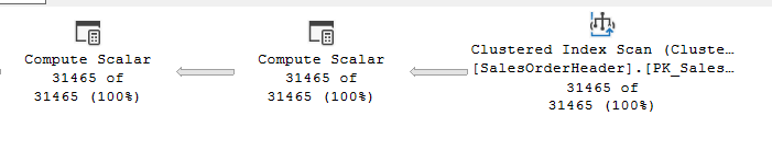
now the estimate is correct and we can see it in dbcc show_statistics like:

DBCC SHOW_STATISTICS('Sales.SalesOrderHeader',_WA_Sys_0000001B_5F7E2DAC)

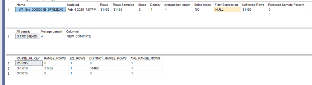
it was the last one created on my device in sys.stats

now if we query the computed column without referencing the new_compute it would still match its

statistics but if it is only a match to the space and the letter, otherwise it would be treated as a different expression

for example:

select*
from Sales.SalesOrderHeader
WHERE Status*SalesOrderID>50000

the estimates are right

but if you write it like this:

select*
from Sales.SalesOrderHeader
WHERE    SalesOrderID * Status  >  50000

we would get the old estimate

Filtered Statistics

is the stats that you create with a predicate in the creation

is the stats that you create with a filtered index

is the stats that you create for a subset of records

why would you do that?

we know the histogram has 200 steps max

sometimes one step has a wild distribution

so we need make the queries run faster on this step

so we create an index or an estimate for that step alone

and we would getter plans

let’s try some

in Sales.SalesOrderHeaderEnlarged:

create statistics subtotal_stats on sales.salesorderheaderenlarged(SubTotal) with fullscan;

then dbcc:

DBCC SHOW_STATISTICS('Sales.SalesOrderHeaderEnlarged',subtotal_stats)

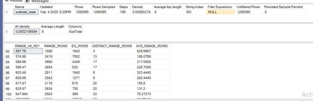
we can see that there are 2419 range_rows with avg_range_rows 217 between 567…. and 574….

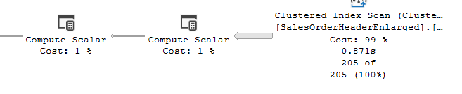
now if we select the following query:

select*
from Sales.SalesOrderHeaderEnlarged
where SubTotal =569.97

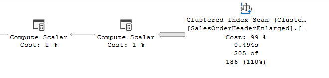
we can see the estimate screwing up for about 10% for this query since the step in the histogram shows that it is 186 even though that it is 205

now if we create filtered stats like:

CREATE STATISTICS SUBTOTAL_FT ON Sales.SalesOrderHeaderEnlarged(SubTotal) 
where SubTotal  >= 567.76
and   SubTotal <=574.98
WITH FULLSCAN

then dbcc it:

dbcc show_statistics('Sales.SalesOrderHeaderEnlarged',SUBTOTAL_FT)

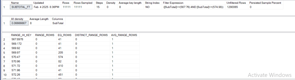
So there are some differences here:

first rows are only the filtered rows not the million something we had in the table

second we see the unfiltered rows here the other rows that do not fit the predicate

now we see 13 more steps

and if we query the query we ran before like:

select*
from Sales.SalesOrderHeaderEnlarged
where SubTotal =569.97

we get an accurate estimate

Ascending Key Statistics

this was an issue of the old cardinality estimator so let’s turn it on for AdventureWorks2022

ALTER DATABASE AdventureWorks2022 SET COMPATIBILITY_LEVEL = 100

Now let’s create a table that has one column:

CREATE TABLE TEST (
COL INT)

now let’s insert 10 values

INSERT INTO TEST (COL)
VALUES 
(1),
(2),
(3),
(4),
(5),
(6),
(7),
(8),
(9),
(10);

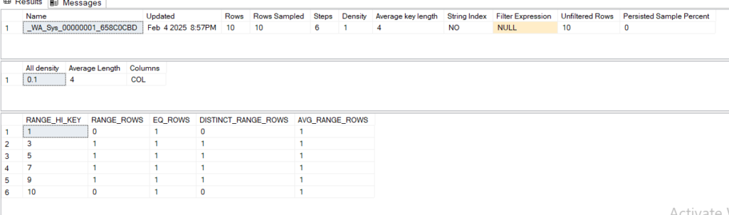
now let’s select to create stats

select* from test where col = 1

let’s dbcc it:

dbcc show_statistics('dbo.test',_WA_Sys_00000001_658C0CBD)

and the output would be

now let’s insert another 5 values :

INSERT INTO TEST (COL)
VALUES 
(11),
(12),
(13),
(14),
(15);

and run the following statement:

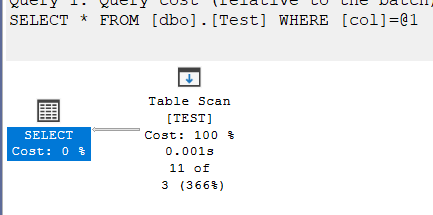
select*
from TEST 
where col>10

and look at the estimate:

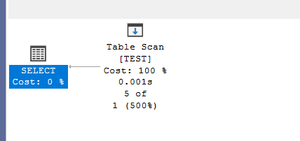
we can see that the estimate is wrong, why?

the new inserted values are not enough for an update

so the stats are outdated

now imagine this was a datetime or identity column, to would have an ever-increasing value, so the stats will always be outdated, to solve that they introduced some trace flags:

Trace flags 2888, 2889

2888 will show us a different set of results for dbcc show_statitistics

2889 would introduce a fix that would update the stats more frequently for this column

so let’s enable both:

DBCC TRACEON (2388)
DBCC TRACEON (2389)

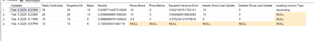
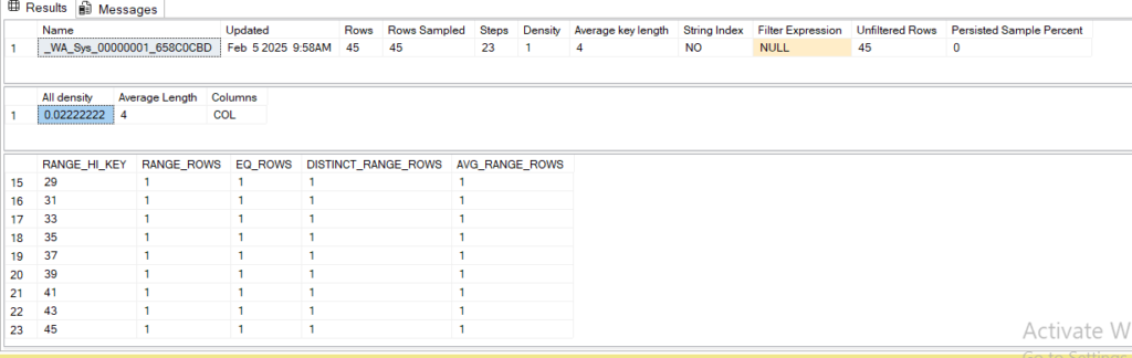
Now let’s run dbcc show_statistics for our stats:

dbcc show_statistics('dbo.test',_WA_Sys_00000001_658C0CBD)

we would see this output:

now if we update stats like:

UPDATE STATISTICS dbo.Test WITH FULLSCAN

Now let’s dbcc again:

so in rows above we had 5.5( i don’t how 5 could be 5 and a half) and 5 inserts 5

now let’s add another 10:

INSERT INTO dbo.test (COL)
VALUES 
(16),
(17),
(18),
(19),
(20),
(21),
(22),
(23),
(24),
(25);

now let’s run our select to see the estimate:

SELECT*
FROM dbo.Test
WHERE COL> 15 

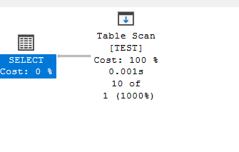
The estimate is still wrong so let’s update the stats again:

UPDATE STATISTICS dbo.Test WITH FULLSCAN

Now let’s dbcc show_statistics:

dbcc show_statistics('dbo.test',_WA_Sys_00000001_658C0CBD)

now the leading column type is still unknown now let’s insert one more time:

INSERT INTO dbo.test (COL)
VALUES 
(26),
(27),
(28),
(29),
(30),
(31),
(32),
(33),
(34),
(35);

now, let’s run our select

SELECT*
FROM dbo.Test
WHERE COL> 25

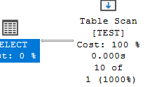
the estimate is still wrong, now let’s update the stats one last time

UPDATE STATISTICS dbo.Test with fullscan

now let’s dbcc it:

dbcc show_statistics('dbo.test',_WA_Sys_00000001_658C0CBD)

the output would be like:

not the key is marked as ascending:

now let’s insert one more last time and look at the select estimates:

INSERT INTO dbo.test (COL)
VALUES 
(36),
(37),
(38),
(39),
(40),
(41),
(42),
(43),
(44),
(45);

now let’s select:

select*
from dbo.Test
where col>35

we still get the wrong estimate

but i updated the stats

but if we insert from 26 to 35 10 times

go
INSERT INTO dbo.test (COL)
VALUES 
(26),
(27),
(28),
(29),
(30),
(31),
(32),
(33),
(34),
(35);
go 10 

then select the following:

select*
from dbo.Test
WHERE COL = 35

why 3 instead of 1: the fix

and we did not even update the stats(which was the whole point of the fix good estimates with no stats update)

now it is using the density information

if we multiply the density information which we would get if opened another session that does not have the traces on we would know that the all density is 0.22

dbcc show_statistics('dbo.test',_WA_Sys_00000001_658C0CBD)

now 0.0222 multiplied by the number of rows which was 45 + 100 = 145

which would be something like = 3.219 or 3

this was without a stats update, this is the improvement, we don’t need it anymore in the new cardinality estimator

now let’s clean up

ALTER DATABASE AdventureWorks2022 SET COMPATIBILITY_LEVEL=160

That would be it for stats, see you in the next blog.