in the previous blog, we talked about logical tree generation

today:

Trivial plan and full optimization
how does SQL Server handle joins
transformation rules
memo

and stuff related to it, most of the trace flags and DMVs are undocumented so we can't use them in a production environment.

Table of Contents

Trivial Plan

since cost-based optimization is an expensive operation, SQL server tries to not use it if it can

when it does that? in trivial plans

what is a trivial plan? it is plan that has one or an obvious best plan from the get go

there is no other way of execution

or this is the best one without much research

so it passes that plan to the execution engine right away for example

USE AdventureWorks2022
BEGIN TRAN 
SELECT Firstname
FROM Person.Person
OPTION(RECOMPILE,QUERYTRACEON 8605,QUERYTRACEON 8606,QUERYTRACEON 8607,
       QUERYTRACEON 8608,QUERYTRACEON 8621,QUERYTRACEON 3604)
COMMIT TRAN

In the output tree:

*** Output Tree: (trivial plan) ***

        PhyOp_NOP

            PhyOp_Range TBL: Person.Person(2) ASC  Bmk ( QCOL: [AdventureWorks2022].[Person].[Person].BusinessEntityID) IsRow: COL: IsBaseRow1000 

********************

or using sys.dm_exec_query_optimizer_info( for ease of use we are going to include the whole code from the previous blog, but you should follow the rules introduced there to get what we get)

use adventureworks2022
BEGIN TRAN
SELECT *
INTO AFTER_OPTIMIZER
FROM sys.dm_exec_query_optimizer_info;
COMMIT TRAN

BEGIN TRAN
SELECT *
INTO BEFORE_OPTIMIZER
FROM sys.dm_exec_query_optimizer_info;
COMMIT TRAN

BEGIN TRAN
DROP TABLE AFTER_OPTIMIZER;
DROP TABLE BEFORE_OPTIMIZER;
COMMIT TRAN

BEGIN TRAN
SELECT *
INTO BEFORE_OPTIMIZER
FROM sys.dm_exec_query_optimizer_info;
COMMIT TRAN

BEGIN TRAN
SELECT PhoneNumberTypeID
FROM Person.PersonPhone
OPTION (RECOMPILE);
COMMIT TRAN

BEGIN TRAN 
SELECT *
INTO AFTER_OPTIMIZER
FROM sys.dm_exec_query_optimizer_info;
COMMIT TRAN 

BEGIN TRAN 
SELECT 
    AFTER_OPTIMIZER.COUNTER,
    (AFTER_OPTIMIZER.OCCURRENCE - BEFORE_OPTIMIZER.OCCURRENCE) AS OCCURRENCE_DIFFERENCE,
    (AFTER_OPTIMIZER.OCCURRENCE * AFTER_OPTIMIZER.VALUE - BEFORE_OPTIMIZER.OCCURRENCE * BEFORE_OPTIMIZER.VALUE) AS VALUE
FROM 
    BEFORE_OPTIMIZER
JOIN 
    AFTER_OPTIMIZER ON BEFORE_OPTIMIZER.COUNTER = AFTER_OPTIMIZER.COUNTER
WHERE 
    BEFORE_OPTIMIZER.OCCURRENCE <> AFTER_OPTIMIZER.OCCURRENCE;
COMMIT TRAN

and this would pop up

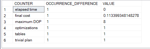
as you can see it is a trivial plan

or we could see in the execution plan xml

SET STATISTICS XML ON;
GO
SELECT PhoneNumberTypeID
FROM Person.PersonPhone
OPTION(RECOMPILE);
GO
SET STATISTICS XML OFF;

click on the XML in the results

...  <BatchSequence>
    <Batch>
      <Statements>
        <...... StatementOptmLevel="TRIVIAL" ...>
          <StatementSetOptions ....>
          <....
</ShowPlanXML>

so it is trivial

or in the execution plan viewer in SSMS

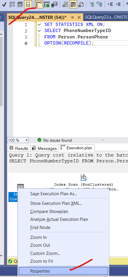
click on show me execution plan the properties on the select operator

and you will see:

now if change the query just a little bit:

SELECT PhoneNumberTypeID
FROM Person.PersonPhone
WHERE PhoneNumberTypeID <> 3
OPTION(RECOMPILE);

and run the test we ran

we would get

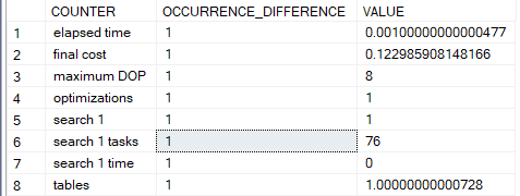
why? inequality predicate

we can disable trivial plans by trace flag 8757

so if we:

SELECT PhoneNumberTypeID
FROM Person.PersonPhone
OPTION(RECOMPILE,QUERYTRACEON 8757);

We will get

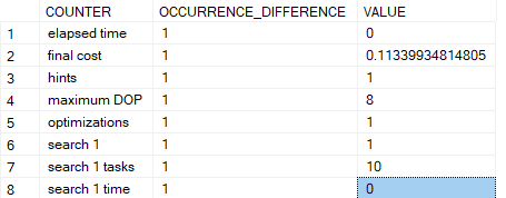
it searched, no trivial plans

Transformation Rules In The Query Optimizer

as we saw in trace flag 8621, SQL server uses certain methods to rewrite a query or a physical operator in the most efficient way, some of them are used during the simplification process, so we call them simplification rules, others are used during the full optimization process. the first one converts the logical tree we had in mind to simpler one like predicate pushdown, so logical to logical, and it does not use cost-based optimization it is just a preparatory phase, transformation on the other hand uses the estimated cost we had through statistics and cardinality estimation to see if the rules could be applied and how useful are they and evaluate the alternatives.

one other type is: Exploration rules. these are cost-based conversion of the simplified logical tree to another one that costs less. so here we are still in logical to logical.

another type of these: Implementation rules. here it would convert the best logical trees it found in the trivial or the cost optimized plans and then convert them to the algorithms that SQL server uses to process the data. for example it might transfer the relational operator LogOp_Join to one of the physical ones like nested loop join.

so what makes a difference between FULL optimization and the trivial plan is the usage of the last two types of rules.

how could we see which rules were applied

sys.dm_exec_query_transformation_stats

first, let’s run select* and see the columns:

SELECT*
FROM  sys.dm_exec_query_transformation_stats

This query shows cumulative results since the last server restart:

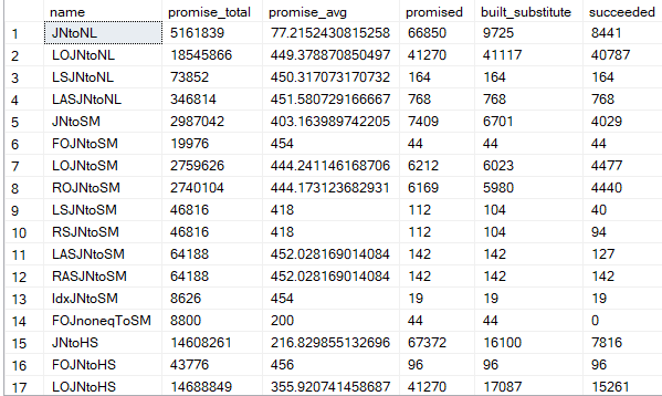
here it shows the:

name: the name of the rule applied for example the first one JNtoNL means a join to a nested loop join, the second one means LOJNtoNL left outer join to a nested loop join, and the third one LSJNtoNL left semi join to a nested loop join
promise_total: how many time the optimizer has been asked to apply this rule
promised: how many times it did actually apply it
built_substitute: how many times it built a substitue physical or logical tree for the rule
succeeded: means how many times it succeeded doing it and added that viable alternative tree to the memo( more on it later)
promise_average: promise_total/promised

so here we can see each rule and how many times it got applied on the whole server,

if we want to see it on a specific query we have to use snapshots just like we did in the previous blog but different columns:

USE AdventureWorks2022;
BEGIN TRAN
SELECT *
INTO AFTER_TRANSFORMATION
FROM sys.dm_exec_query_transformation_stats;
COMMIT TRAN

BEGIN TRAN
SELECT *
INTO BEFORE_TRANSFORMATION
FROM sys.dm_exec_query_transformation_stats;
COMMIT TRAN

BEGIN TRAN
DROP TABLE AFTER_TRANSFORMATION;
DROP TABLE BEFORE_TRANSFORMATION;
COMMIT TRAN

BEGIN TRAN
SELECT *
INTO BEFORE_TRANSFORMATION
FROM sys.dm_exec_query_transformation_stats;
COMMIT TRAN

SELECT PhoneNumberTypeID
FROM Person.PersonPhone
OPTION(RECOMPILE);

BEGIN TRAN
SELECT *
INTO AFTER_TRANSFORMATION
FROM sys.dm_exec_query_transformation_stats;
COMMIT TRAN

BEGIN TRAN;
SELECT 
    AFTER_TRANSFORMATION.name,
    (AFTER_TRANSFORMATION.promised - BEFORE_TRANSFORMATION.promised) AS PROMISED
FROM 
    BEFORE_TRANSFORMATION
JOIN 
    AFTER_TRANSFORMATION ON BEFORE_TRANSFORMATION.name = AFTER_TRANSFORMATION.name
WHERE 
    BEFORE_TRANSFORMATION.succeeded <> AFTER_TRANSFORMATION.succeeded;
COMMIT TRAN;

and the output would be:

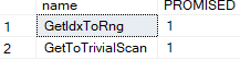
so here it basically did these two once each:

GetidxToRng: so here it converted the get index meaning the index seek to an index range scan, since it was more efficient to retrive all the phone ids instead of seeking each one separately

GetToTrivialScan: here it says it converted the get logical operator to the trivial scan, our trivial plan’s table scan since it needed all the rows from the table

now let’s disable the trivial and run it again:

SELECT PhoneNumberTypeID
FROM Person.PersonPhone
OPTION(RECOMPILE,querytraceon 8757,querytraceon 8619,querytraceon 8620,querytraceon 3604)

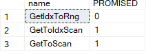
now here it optimized and:

GetIdxToRng: it converted the logical get index to a range but it never even tried to complete it
GetToIdxScan: it converted the get logical to an index scan
GetToScan: it converted the get logical to a table scan logical

now for the output of the trace flags:

---------------------------------------------------

Apply Rule: GetToScan - Get()->Scan()
    Args: Grp 0 0 LogOp_Get (Distance = 0)

---------------------------------------------------

Apply Rule: GetToIdxScan - Get -> IdxScan
    Args: Grp 0 0 LogOp_Get (Distance = 0)

it does not show the first one, since it never got executed

it shows the second and the third

and shows the memo stuff that we will talk about later

now if we use a where clause

SELECT PhoneNumberTypeID
FROM Person.PersonPhone
WHERE PhoneNumberTypeID<> 3
OPTION(RECOMPILE,querytraceon 8619,querytraceon 8620,querytraceon 3604)

And the traces:

---------------------------------------------------

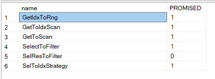
Apply Rule: SelToIdxStrategy - Sel Table -> Index expression 
    Args: Grp 4 0 LogOp_Select 3 2 (Distance = 0)
---------------------------------------------------

Apply Rule: GetIdxToRng - GetIdx -> Rng
    Args: Grp 5 0 <SelToIdxStrategy>LogOp_GetIdx (Distance = 1)

---------------------------------------------------

Apply Rule: SelectToFilter - Select()->Filter()
    Args: Grp 4 0 LogOp_Select 3 2 (Distance = 0)

---------------------------------------------------

Apply Rule: GetToScan - Get()->Scan()
    Args: Grp 3 0 LogOp_Get (Distance = 0)

---------------------------------------------------

Apply Rule: GetToIdxScan - Get -> IdxScan
    Args: Grp 3 0 LogOp_Get (Distance = 0)

so the first says use an index

the second says instead of an index use a table or range scan

the third is don’t select immediately filter first

the fourth converts the get to a table scan

the 5th says convert the get to a scan

so it considered each of these and then, it used the idxscan at the end based on the cost

so these are some of the rules and how could we explore them

we could explore a more complicated query:

SELECT P.ProductID,COUNT(*)
FROM Production.Product P INNER JOIN Production.ProductInventory I 
                            ON P.ProductID = I.ProductID
GROUP BY P.ProductID
OPTION(RECOMPILE,QUERYTRACEON 8606,QUERYTRACEON 8607,
QUERYTRACEON 8608,QUERYTRACEON 3604,
QUERYTRACEON 8619,QUERYTRACEON 8620,
QUERYTRACEON 8621,QUERYTRACEON 8615,
QUERYTRACEON 8675)

The DMV:

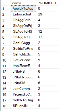
A lot of rules.

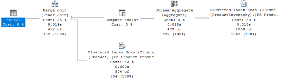
most authors focus on GbAggBeforeJoin because it is in the execution plan and reduces resource consumption a lot, so we are going to explain it first:

so here in the group by we specified P.ProductID, and it already exists in the P table

so instead of joining and then later group by it, we can filter the results by it, then after that, we could produce the output thus reducing cost

inGbAggToStAgg: it converts the group by aggregate function to a stream aggregate

in the GetToIdxScan it converts the get logical operator to an index scan

in JoinCommute it uses the commutativity rule in which a join b = b join a

in JNtoSM it converts a join to a merge join

and in the execution plan, we can see each of these

So, it first converted the logical to physical, compared the results of each based on statistics, and then started converting to physical operators. After that, it compared the estimated results and chose the best one.

if we look up the total cost in the execution plan:

now if we disable some rules like GbAggBeforeJoin using the code provided below:

DBCC RULEOFF('GbAggBeforeJoin')

and run the query again:

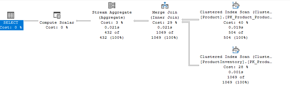
the stream aggregate happened after the join and the cost would be 0.0314982 so there is a slight increase

now if we disable the

DBCC RULEOFF ('GbAggToStrm')

Then execute:

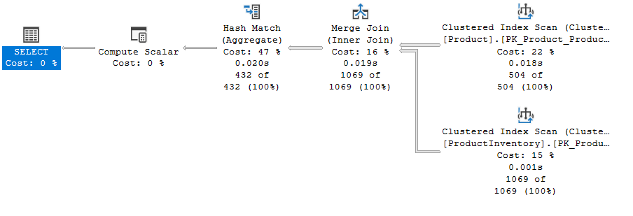
so it used GbAggToHS and the cost 0.0579313 almost doubled now if we disable that

DBCC RULEOFF ('GbAggToHs')

And execute we would get this error


Query processor could not produce a query plan because of the hints defined
 in this query. Resubmit the query without specifying any
  hints and without using SET FORCEPLAN.

so now since the the optimizer can not convert the group by to a physical operator

now we can turn them on by:

DBCC RULEON ('GbAggToHs') ;
DBCC RULEOn('GbAggToStrm') ;
DBCC RULEOn('GbAggBeforeJoin') ;

and our query will return to its original shape

Memo

when SQL Server tries to explore the alternative plans for a query, it stores them in the memo.

these could be logical or physical ones.

each optimization has its own memo.

if the query did not go through optimization, meaning it was trivial it would not be there

if it did go through the process and got some transformation rules applied on it, it would have a memo.

the memo does not store each and every step, it recognizes similarities groups them, and stores them in an efficient way.

the costs of each physical alternative are stored, then the lower one wins.

let’s explore it

we have two trace flags to show us the structure: 8608 for the initial and 8615 for the final one assuming trace flag 3604 is enabled.

we’ll look at a trivial plan, then disable it using 8757

then look at some fully optimized plan, and see how it is stored in the memo.

so first:

BEGIN TRAN 
SELECT ProductID
FROM Production.Product
OPTION(RECOMPILE,QUERYTRACEON 3604,QUERYTRACEON 8608, QUERYTRACEON 8615)
COMMIT TRAN

As you can see no output

now let’s disable trivial plan using 8757:

BEGIN TRAN 
SELECT ProductID
FROM Production.Product
OPTION(RECOMPILE,QUERYTRACEON 8757,QUERYTRACEON 3604,QUERYTRACEON 8608, QUERYTRACEON 8615)
COMMIT TRAN

And the output would be:

--- Initial Memo Structure ---

Root Group 0: Card=504 (Max=10000, Min=0)

   0 LogOp_Get (Distance = 0)

------------------------------

--- Final Memo Structure ---

Root Group 0: Card=504 (Max=10000, Min=0)

   2 PhyOp_Range 4 ASC   Cost(RowGoal 0,ReW 0,ReB 0,Dist 0,Total 0)= 0.00457714 (Distance = 1)

   0 LogOp_Get (Distance = 0)

----------------------------

so first it has its root group which is 0

it has a cardinality estimation of 504

it contains the Logical operator Get

this operator’s identifier is 0

so whenever SQL Server sees 0 in this plan it would be LogOp_Get

Distance: how many steps did the optimizer use to get to this specific operator

now in the final memo, we see an additional physical operator

it has one group

it is the initial root group

it contains two operators

PhyOp_Range which is identified as 2 and it has a distance of 1 meaning the optimizer needed one step to find it

the initial with no optimization operator 0

now if we run a non-trivial plan:

BEGIN TRAN 
SELECT ProductID
FROM Production.Product
where ProductID <> 3
OPTION(RECOMPILE,QUERYTRACEON 3604,QUERYTRACEON 8608,QUERYTRACEON 8609, QUERYTRACEON 8615)
COMMIT TRAN

and the output

--- Initial Memo Structure ---

Root Group 4: Card=503 (Max=10000, Min=0)

   0 LogOp_Select 3 2 (Distance = 0)

Group 3: Card=504 (Max=10000, Min=0)

   0 LogOp_Get (Distance = 0)

Group 2: 
   0 ScaOp_Comp  0 1 (Distance = 0)

Group 1: 
   0 ScaOp_Const  (Distance = 0)

Group 0: 
   0 ScaOp_Identifier  (Distance = 0)

so we have:

the root group which was the first group to be explored
it has one logical operator identified as 0 and it references the other groups 3 and 2
now in 3 we see the cardinality estimation which is 504, it has one logical operator that does not reference anything which is the LogOp_Get which is basically a select and it did not explore much to get it
in 2 we see the ScaOp_Comp it is group by distance( as depicted in the output of 8609) and it has one operator that references 0 and meaning it checks if the identifier equals the constant
in group 1 we see the ScaOp_Const which corresponds to the 3 we queried
in 0 we see the ScaOp_Identifer which verifies that we have the correct row from the correct table
so the plan has the first logOp_select has a get that uses a comparison operator who looks if the row we want does not equal 3

then in the output of 8609:

Tasks executed: 34
Rel groups: 2
Log ops: 2
Phy ops: 0
Sca groups: 3
Sca ops: 3
Total log ops: 2
Count of log ops, grouped by exploration distance
 0: 2
Total phy ops: 0
Count of phy ops, grouped by exploration distance
Total sca ops: 3
Count of sca ops, grouped by exploration distance
 0: 3

it shows what it did to get the initial memo plus optimize it

so it has 2 relational groups = LogOp operators

0 physical still playing with logical

3 scalar groups

then it counts and groups them

then in the final memo:


--- Final Memo Structure ---

Group 8: 
   0 ScaOp_Logical  6.0 7.0  Cost(RowGoal 0,ReW 0,ReB 0,Dist 0,Total 0)= 7 (Distance = 1)
Group 7: 
   0 ScaOp_Comp  0.0 1.0  Cost(RowGoal 0,ReW 0,ReB 0,Dist 0,Total 0)= 3 (Distance = 1)
Group 6: 
   0 ScaOp_Comp  0.0 1.0  Cost(RowGoal 0,ReW 0,ReB 0,Dist 0,Total 0)= 3 (Distance = 1)
Group 5: Card=504 (Max=10000, Min=0)
   1 PhyOp_Range 2 ASC   Cost(RowGoal 0,ReW 0,ReB 0,Dist 0,Total 0)= 0.00457714 (Distance = 2)
   0 LogOp_GetIdx (Distance = 1)
Root Group 4: Card=503 (Max=10000, Min=0)
   1 PhyOp_Filter 5.1 8.0  Cost(RowGoal 0,ReW 0,ReB 0,Dist 0,Total 0)= 0.00502066 (Distance = 1)
   0 LogOp_Select 3 2 (Distance = 0)
Group 3: Card=504 (Max=10000, Min=0)
   0 LogOp_Get (Distance = 0)
Group 2: 
   0 ScaOp_Comp  0 1 (Distance = 0)
Group 1: 
   0 ScaOp_Const   Cost(RowGoal 0,ReW 0,ReB 0,Dist 0,Total 0)= 1 (Distance = 0)
Group 0: 
   0 ScaOp_Identifier   Cost(RowGoal 0,ReW 0,ReB 0,Dist 0,Total 0)= 1 (Distance = 0)

The ReW and Reb are rewinds and rebinds( more on them in another blog)

Groups 0, 1, 2, 3 are the same
root group 4 added a physical operator now, PhyOp_Filter that references 5 and 1 so it filters on 5 and 1 or it filters on 8 and 0
then it shows the cost
group 5: it has the scanning range operator in asc way so an index scan referencing group 2 which is the comparison operator, and one GetIdx operator
group 6: has a comparison operator that references 0 and 0 or 0 and 1 so it is like group 2 in terms of comparing the identifier to the constant
group 7: did the same
group 8: combines 8 and 7 in one scalar

so the root group is the chosen plan, which was the original one.

we did not see any other physical alternative in here

now for the output of 8609 for the final memo:

Tasks executed: 66
Rel groups: 3
Log ops: 3
Phy ops: 2
Sca groups: 6
Sca ops: 6
Total log ops: 3
Count of log ops, grouped by exploration distance
 0: 2
 1: 1
Total phy ops: 3
Count of phy ops, grouped by exploration distance
 0: 0
 1: 2
 2: 1
Total sca ops: 6
Count of sca ops, grouped by exploration distance
 0: 3
 1: 3

so it added the physicals and the search distance says which type of search it did is it search 0, 1, or 2

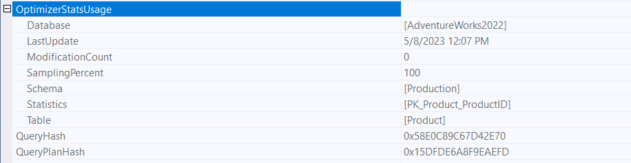
Statistics

in order for SQL Server to optimize a query, it needs to compare costs

and in order to do that you need to know the data in the table

now since you can’t access all the data every time you tune a query you need a sample

based on this sample .SQL server tries to create an optimized plan if it is necessary ( not trivial)

it contains information on the distribution of values across columns, indexes, etc.(more on it in another blog)

we can see that in the properties of the execution plan in optimizer stats usage:

or we could use trace flags 9292 and 9204

both only work on the legacy cardinality estimator so we have to enable it first then show it

use adventureworks2022
ALTER DATABASE SCOPED CONFIGURATION
SET LEGACY_CARDINALITY_ESTIMATION = ON

Now:

BEGIN TRAN 
SELECT ProductID
FROM Production.Product
where ProductID <> 3
OPTION(RECOMPILE,QUERYTRACEON 3604,QUERYTRACEON 9292,QUERYTRACEON 9204)
COMMIT TRAN

and the output would be:

Stats header loaded: DbName: AdventureWorks2022, 
ObjName: Production.Product, IndexId: 1, ColumnName: ProductID, EmptyTable: FALSE

Stats loaded: DbName: AdventureWorks2022, 
ObjName: Production.Product, IndexId: 1, ColumnName: ProductID, EmptyTable: FALSE

now let’s create some statistics objects:

CREATE STATISTICS ProductID_Stats ON Production.Product (ProductID);

now let’s run the query again:

Stats header loaded: DbName: AdventureWorks2022,
 ObjName: Production.Product, IndexId: 1, ColumnName: ProductID, EmptyTable: FALSE

Stats loaded: DbName: AdventureWorks2022, 
ObjName: Production.Product, IndexId: 1, ColumnName: ProductID, EmptyTable: FALSE

Stats header loaded: DbName: AdventureWorks2022, 
ObjName: Production.Product, IndexId: 9, ColumnName: ProductID, EmptyTable: FALSE

so now we can see how many stats we have, we can drop them:

DROP STATISTICS Production.Product.ProductID_Stats

now it will be cleared, let’s run the new cardinality estimator again

use adventureworks2022
ALTER DATABASE SCOPED CONFIGURATION
SET LEGACY_CARDINALITY_ESTIMATION = off

FULL Optimization process:

now we know about the rules, memo, trivial plans, and stats.

how does SQL Server use the following to optimize a plan?

so if the plan is trivial = no optimization = none of this is necessary

but if it is:

there are a lot of execution plans that could be generated for each plan, sometimes it could be millions.

so does SQL Server search the millions and then take the best one? no, it does not

instead it costs the logical operators generated, and applies rules if the cost could be reduced by them.

how? Heuristic algorithms know if a specific rule could reduce the cost or not

if it does, then it gets applied and costs the logical alternative plans at each generation

if one of them costs a lot, the other alternatives that come through that plan will be discarded

and it will focus on the cheapest. then it re-iterates the process and generates alternatives for the subnodes of the cheapest and if one of them even remotely looks expensive it gets discarded and it only focuses on the cheapest one…….. until either a good enough plan gets generated.

if it finds one then it presents it.

if not then there are two options, it either stops the process since it has a limit on time that could be spent on each step, or it could move to a higher level of algorithms if the plan looks more complex than it seemed at first look, now if the plan goes the other search it could get generated in time so a good enough plan will be there, or it could time_out and the reason for termination of the optimization process would be not enough time.

there are 3 phases of optimization: search 0, 1, and 2 which are the distance in the previous trace flags.

we can see the phases using sys.dm_exec_query_optimizer_info.

Search 0 (transaction processing)

it is the first phase of optimization, used for simple OLTP queries

it would try to find a plan as quickly as possible

it needs at least 3 tables

before the optimization, it generates the joins required

looks which one would be the cheapest to join first using the commutativity and associativity rules

then it starts with the smallest or the most selective

then it starts looking for the cheapest physical operators

it keeps on going until it finds a good enough plan based on that statistics

or it times out

or it moves to another phase if the query looks more complex now

for example:

SELECT E.JobTitle, P.PayFrequency, COUNT(E.JobTitle)
FROM HumanResources.Employee E inner join HumanResources.EmployeePayHistory P
                               ON E.BusinessEntityID = P.BusinessEntityID
                               INNER JOIN HumanResources.EmployeeDepartmentHistory D
                               ON E.BusinessEntityID = D.BusinessEntityID
group by  E.JobTitle, P.PayFrequency
OPTION(RECOMPILE,querytraceon 3604)

We would get

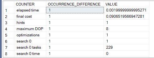
so it searched in 0 1 time the value was 229

Search 1 (quick plan)

it uses additional transformation rules

some join reordering

In the end, it compares the cost to the internal cost threshold

if it matches it or below then a good enough plan is generated

if not , it looks if a parallel query is necessary

if it could be generated it would generate the parallel plans

then it compares their costs to the serial plan

and picks the cheapest one

then it uses it in the next phase which is Search 2

for example:

SELECT*
FROM HumanResources.Employee
WHERE NationalIDNumber <> 50 
OPTION (RECOMPILE)

the output of the DMV would be:

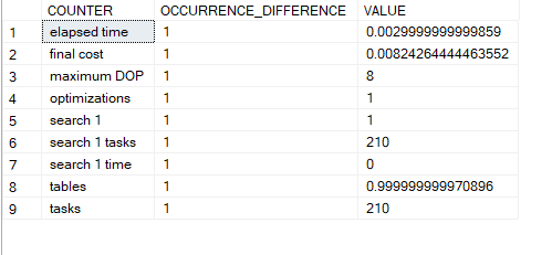
went to search 1 right away

Now it could search 0 first then move on to search 1 for example:

SELECT DISTINCT 
    p.ProductID,
    p.Name AS ProductName,
    wor.ScheduledStartDate,
    e.JobTitle
FROM 
    Production.WorkOrder wo
JOIN 
    Production.WorkOrderRouting wor ON wo.WorkOrderID = wor.WorkOrderID
JOIN 
    Production.Product p ON wor.ProductID = p.ProductID
JOIN 
    HumanResources.Employee e ON wo.StockedQty = e.BusinessEntityID  -- Example join condition
WHERE 
    p.ProductID = 800
OPTION 
    (RECOMPILE,QUERYTRACEON  3604, QUERYTRACEON 8675);

and the output would be:

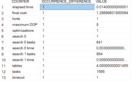
now here i first went through 0

did not suffice

went through 1

but the query took to long to be processed

so it timed out

it could not show us any gain from going through 1

but it might and then it would show us how much it saves from it

but here it costs more to go through the search one since it costs 0.005 instead of 0.003

In the trace output:

End of simplification, time: 0.001 net: 0.001 total: 0.001 net: 0.001

end exploration, tasks: 227 no total cost time: 0.003 net: 0.003 total: 0.004 net: 0.004

end search(0),  cost: 1.299 tasks: 641 time: 0.005 net: 0.005 total: 0.01 net: 0.01

end exploration, tasks: 1234 Cost = 1.299 time: 0.002 net: 0.002 total: 0.012 net: 0.012

*** Optimizer time out abort at task 1595 ***

end search(1),  cost: 1.299 tasks: 1595 time: 0.001 net: 0.001 total: 0.014 net: 0.014

*** Optimizer time out abort at task 1595 ***

End of post optimization rewrite, time: 0 net: 0 total: 0.014 net: 0.014

End of query plan compilation, time: 0 net: 0 total: 0.014 net: 0.014

here it shows what we just explained

Search 2:( full optimization)

this is designed for complex to very complex queries.

more transformation rules

more parallel operators

advanced strategies

for example:

SELECT 
    soh.SalesPersonID,
    st.Name AS TerritoryName,
    p.Name AS ProductName,
    sod.LineTotal,
    SUM(sod.LineTotal) OVER (PARTITION BY soh.SalesPersonID ORDER BY soh.OrderDate ROWS BETWEEN UNBOUNDED PRECEDING AND CURRENT ROW) AS RunningTotalSales,
    RANK() OVER (PARTITION BY soh.TerritoryID ORDER BY SUM(sod.LineTotal) DESC) AS SalesRank
FROM 
    Sales.SalesOrderHeader soh
JOIN 
    Sales.SalesOrderDetail sod ON soh.SalesOrderID = sod.SalesOrderID
JOIN 
    Production.Product p ON sod.ProductID = p.ProductID
JOIN 
    Sales.SalesTerritory st ON soh.TerritoryID = st.TerritoryID
JOIN 
    HumanResources.Employee e ON soh.SalesPersonID = e.BusinessEntityID
JOIN 
    Person.Person pe ON e.BusinessEntityID = pe.BusinessEntityID
GROUP BY 
    soh.SalesPersonID, 
    st.Name, 
    p.Name, 
    sod.LineTotal, 
    soh.OrderDate,
    soh.TerritoryID
ORDER BY 
    SalesRank option ( recompile,querytraceon 3604,querytraceon 8675, querytraceon 2372)

and the output:

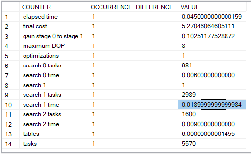
so here it went through all the phases 0, 1, and 2

it shows us the gain stage 0 to stage 1 which means there 10 percent decrease in cost

if we look up the output of our trace flags first 8675:

End of simplification, time: 0.001 net: 0.001 total: 0.001 net: 0.001

end exploration, tasks: 238 no total cost time: 0.004 net: 0.004 total: 0.006 net: 0.006

end exploration, tasks: 243 no total cost time: 0 net: 0 total: 0.006 net: 0.006

end search(0),  cost: 5.87246 tasks: 981 time: 0.003 net: 0.003 total: 0.009 net: 0.009

end exploration, tasks: 1755 Cost = 5.87246 time: 0.003 net: 0.003 total: 0.012 net: 0.012

end exploration, tasks: 1761 Cost = 5.87246 time: 0 net: 0 total: 0.012 net: 0.012

end search(1),  cost: 5.27046 tasks: 3970 time: 0.011 net: 0.011 total: 0.026 net: 0.026

end exploration, tasks: 4546 Cost = 5.27046 time: 0.002 net: 0.002 total: 0.028 net: 0.028

end exploration, tasks: 4553 Cost = 5.27046 time: 0 net: 0 total: 0.029 net: 0.029

end search(2),  cost: 5.27046 tasks: 5570 time: 0.003 net: 0.003 total: 0.033 net: 0.033

End of post optimization rewrite, time: 0 net: 0 total: 0.033 net: 0.033

End of query plan compilation, time: 0.001 net: 0.001 total: 0.035 net: 0.035

as you can see at the end of stage 2 it did not decrease the cost so no gain there, it did not time out it just chose the same plan

but it decreased the cost from stage 0 to 1 which was the gain from 5.87246 to 5.27046 which is like 10 percent

we can see how much memory it used, how long did it take, in each step

for 2372:

Memory before NNFConvert: 28

Memory after NNFConvert: 28

Memory before project removal: 31

Memory after project removal: 34

Memory before simplification: 34

Memory after simplification: 81

Memory before heuristic join reordering: 81

Memory after heuristic join reordering: 91

Memory before project normalization: 91

Memory after project normalization: 96

Memory before stage TP: 116

Memory after stage TP: 157

Memory before stage QuickPlan: 157

Memory after stage QuickPlan: 210

Memory before stage Full: 210

Memory after stage Full: 241

Memory before copy out: 242

Memory after copy out: 246

so here we can see how much memory it used at each step, it did store in the memo the alternative search 2 plan, it just did not use it

here we can’t see the reason for early termination in the execution plan, XML, or anywhere

my guess it went through Phase 2 it did not find a parallel plan but it saved cost during phase 1, it looked in the time_out limit of Phase 2 so it did not exceed it, but the parallel plan was not better than Phase 1 plan so it did not include an output.

after that the estimated execution plan will be passed to the execution engine

and that would be the end of the query optimization part 2.

see you later.

One response to “Query Optimizer In SQL Server: Part 2 Physical Operators”

Multiple Distincts In A Query: Execution Engine Part 2 - Suleyman Essa says:

April 9, 2025 at 3:44 pm

[…] the transformation rules that has been implemented since the restart of the server, we introduced here. here we are going to take some snapshots of the query before and after the query, so we could know […]

Trivial Plan

Transformation Rules In The Query Optimizer

sys.dm_exec_query_transformation_stats

Memo

Statistics

FULL Optimization process:

Search 0 (transaction processing)

Search 1 (quick plan)

Search 2:( full optimization)

One response to “Query Optimizer In SQL Server: Part 2 Physical Operators”

Leave a Reply Cancel reply

Quick Links

Get In Touch