In the previous two blogs, we introduced two physical implementations of joins in SQL Server: nested loop join and a merge join.

Today we are going with the third:

Intro

When it comes to smaller datasets, nested loops exceed,

In medium-sized datasets, we get the merge if we want

For a larger dataset, the best algorithm and the most scalable.

It requires at least one equijoin predicate, residual predicates, and all kinds of semi and outer joins

The algorithm

We quote Craig Freedman:

for each row R1 in the build table
begin
calculate hash value on R1 join key(s)
insert R1 into the appropriate hash bucket
end
for each row R2 in the probe table
begin
calculate hash value on R2 join key(s)
for each row R1 in the corresponding hash bucket
if R1 joins with R2
return (R1, R2)
end

So:

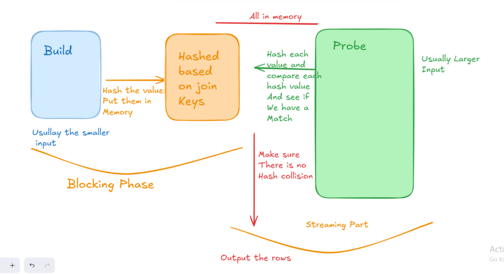
We have two tables, build and probe

Now the algorithm does not execute until it builds the build, usually the smaller table, so it read all the rows from the first table, R1, left or build, hashes, meaning, calcutlating a hash value, meaning, it does some calcutlation that converts the data we have, no matter what it is, to a key, that is usually numerical or hexidecimal, then after it builds the first input, then in the probe phase, or the probe table, it starts reading after hashing, each row, to process it according to the join predicate, and looks for matches using the hash,

So after it finishes the build, it goes to the probe and looks for equavilants, and it does that using the hashing calcutlations.

While building, it is a blocking process, but once the build phase is done, it start streaming.

Now, we can have hash collisions, meaning two different rows having the same hash values. we must check each potential match after the hash is done.

The hashing is done in memory, or in a worktable in tempdb if there are not enough grants and there is some spillage

So we have to give memory to each hash join, meaning the more you have, the more memory you need, meaing there is a limit on how many hash joins you can have in a system, now this not might not be an issue for BI level data, since we are running few queries at once, this could lead to resource consumption in an OLTP database system, and that is why we have other join algoirthms for smaller datasets.

Spilling

Now, like we said, if there is not enough memory grant estimated, we start to spill

Meaning, we usually collect similar hash values in buckets, now if the optimizer guessed right, we get what we want, joining in memory,

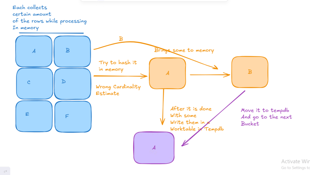
but if the optimizer failed to estimate the value, it had to process each bucket individually, store in tempdb, get another bucket, put it in memory, process it, then store that in tempdb, then do that until it finishes the build, now if it encounters a row that belongs to another bucket, it writes it to its bucket in tempdb

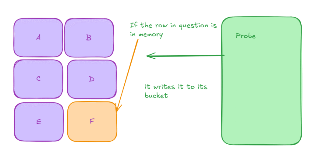
Now, in the probe phase, it looks at the hashed value; if it is in memory, we are golden

Now, if the row is in tempdb, it probes it in the disk table

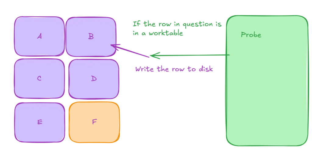
After all the probing is done, it starts writing the buckets one by one to memory

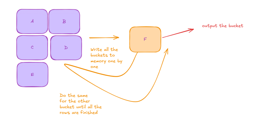
This makes the operation a lot more slower

Join trees used in a hash join

Now, we can consider the joins in question in multiple forms, each of which has certain limitations

For example, a bushy join:

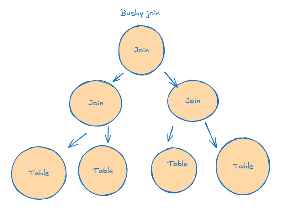
Considers all alternatives, gets the best way of execution, which increases the exploration time of multiple joins, making it longer for the optimizer to construct a query, but it gets the best plan out there

And there are two other types:

Now, these two other alternatives may not come with the best alternative, but they require way less time to conduct the search for a good enough plan

Now, this is significant in query optimization,

We know that SQL Server uses a left deep plan, and that is equivalent to the right deep in terms of optimization, commutativity, and associativity

What about hash joining? How does that affect it? memory

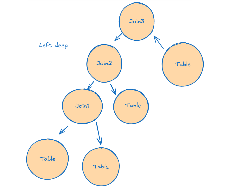
Each join in a left deep tree is the build for the next, so the less the join output is, the faster the probing, the less memory we use

This figure:

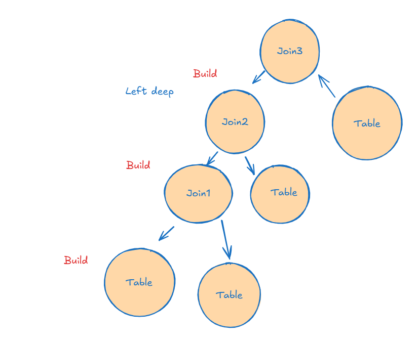
The smaller table at first is the build

Join1 is the build for the second join

Join2 is the build for the third join

And the probing is blocked by building the previous table

So we have to store it in memory the first build table, until we finish the join1

Once we finish the probing the first join, we can release the table from memory( the first build table)

After that, we have to keep the join1 in memory while probing until we finish Join2

After that, we release join1 and use join2 to probe against the last table in join3

So there is a wait for finishing the probe, and we have to store JOIN1 and JOIN2 while probing it, so this could be the max memory grant

Or it could be while probing JOIN2 with JOIN3

So the max could be Join1 + Join2 or Join2 + Join3

This is the left deep tree

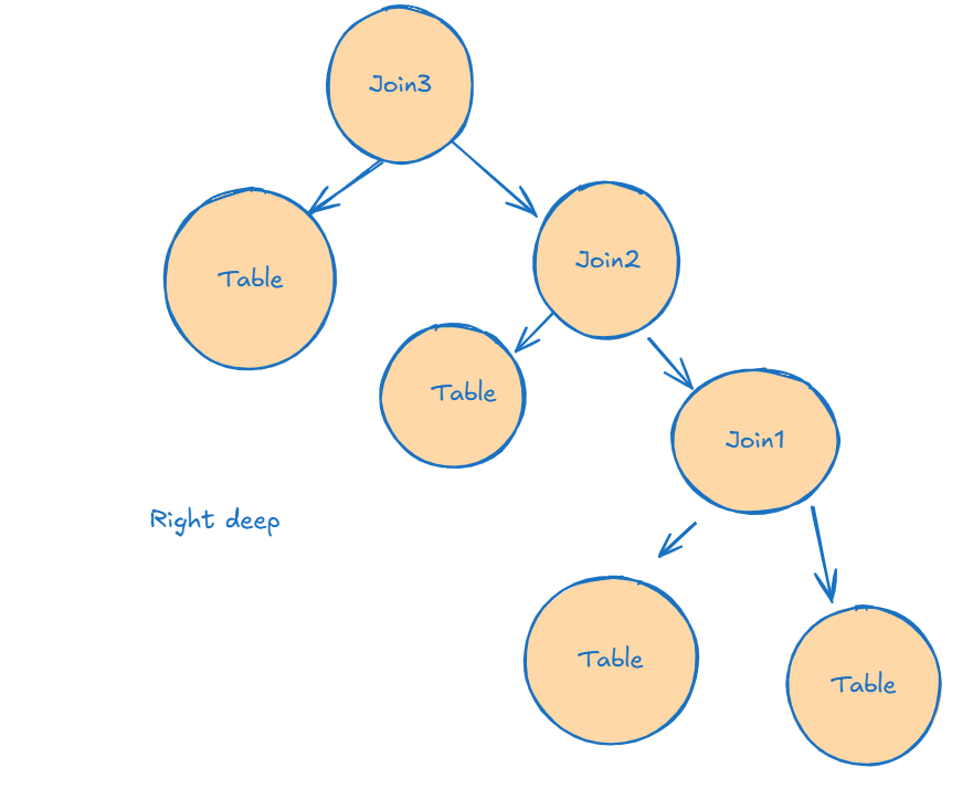
In a right deep tree, we can’t do that, we have to build all the tables before probing, thus making the max Join1+Join2+Join3

Let’s do some demos

Demos

use adventureworks2022
go
create table hash1 (
col1 int,
col2 int,
St char(100)
);
go
create table hash2(
col1 int,
col2 int,
st char(100)
);
go
create table hash3(
col1 int,
col2 int,
st char(100)
)
go
with
n1(c) as (select 0 union all select 0 ),
n2(c) as ( select 0 from n1 as t1 cross join n1 as t2),
n3(c) as ( select 0 from n2 as t1 cross join n2 as t2),
n4(c) as (select 0 from n3 as t1 cross join n3 as t2),
ids(id) as (select ROW_NUMBER() over (order by (select null)) from n4)
insert into hash1(col1,col2)
select id,id 
from ids;
go 4
with
n1(c) as (select 0 union all select 0 ),
n2(c) as ( select 0 from n1 as t1 cross join n1 as t2),
n3(c) as ( select 0 from n2 as t1 cross join n2 as t2),
n4(c) as (select 0 from n3 as t1 cross join n3 as t2),
ids(id) as (select ROW_NUMBER() over (order by (select null)) from n4)
insert into hash2(col1,col2)
select id,id 
from ids;
go 40
go
with
n1(c) as (select 0 union all select 0 ),
n2(c) as ( select 0 from n1 as t1 cross join n1 as t2),
n3(c) as ( select 0 from n2 as t1 cross join n2 as t2),
n4(c) as (select 0 from n3 as t1 cross join n3 as t2),
ids(id) as (select ROW_NUMBER() over (order by (select null)) from n4)
insert into hash3(col1,col2)
select id,id 
from ids;
go 400

Now, in this setup we have 3 tables with approximately 1,000, 10 000, 100 000 rows

So, we can probe by each

:

select*
from hash1 inner join hash2 on hash1.col1= hash2.col1

We get:

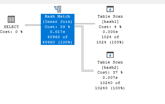
Now, in the properties:

As you can see, it chose hash1 as the build since it has fewer rows

If we do the following:

select*
from hash1 inner join hash2 on hash1.col1 = hash2.col1
           inner join hash3 on hash2.col1 = hash3.col1

We get:

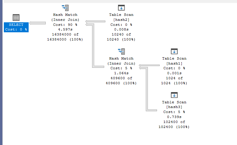
As you can see, it chose the hash one as a probe for the hash 3 since it is way too low, and the number of hash 3 is way too high, if we force orde of what we need, we get an increase in cost, since it would have more rows in build, since it have to be more rows in the second, it chose the to build by the first,

If the tree was a left deep one, it decreased the memory consumption by choosing the least count of the two combinations

If it was a right deep tree, then it chose one, that might introduce some overhead, if it matched the combination as specified by the order of joins, but it decreased the execution time by building the smaller tables

What would happen if we add a predicate to restrict the row count like:

select*
from hash1 inner join hash2 on hash1.col1 = hash2.col1
           inner join hash3 on hash2.col1 = hash3.col1
where hash2.col1<100

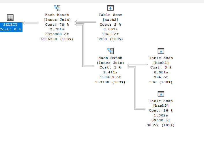
As you can see here, it reduced the count of rows to 1/3, which makes the query quicker, but not much changed here since the query optimizer reordered our joins

In both cases, we used a right deep plan, which had to store and build all the builds before starting to execute the query

And with that, we finish this intro blog on hash joins. see you in the next one.