Now, in the previous blogs, we explored some of the physical operators of implementing aggregations, showed their effects on subqueries. still, most of the aggregations were too simple, Today, we will use a new way of grouping that could produce more useful results, so we could step up our game a little bit, not too much, so tag a long.

Table of Contents

Query

For example:

use adventureworks2022;
go
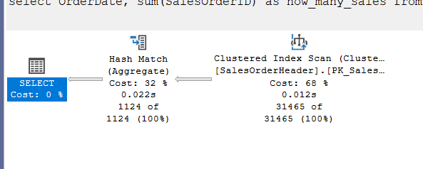
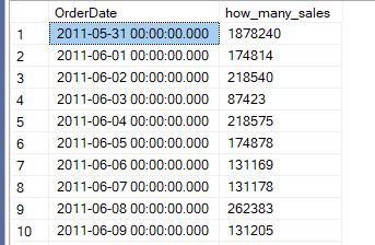
select OrderDate, sum(SalesOrderID) as how_many_sales
from Sales.SalesOrderHeader
group by OrderDate
go

Now, here we are trying to know how many sales there were by order date, simple aggregation, since we did not request a specific order, the input is a little too much, and there is no index. SQL Server chose a hash aggregate like we explained before:

Now, even if I wanted the order like:

go
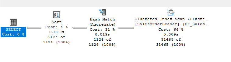
select OrderDate, sum(SalesOrderID) as how_many_sales
from Sales.SalesOrderHeader
group by OrderDate
order by OrderDate
go

We would get a hash with a sort after, since it is less costly to aggregate and then sort:

How to force a stream aggregate(option(order group))

Now, if you want to force the grouping by groups, regardless of the order, meaning: I want my groups sorted before aggregating, we would get our plan:

go        
select OrderDate, sum(SalesOrderID) as how_many_sales
from Sales.SalesOrderHeader
group by OrderDate
option(order group)
go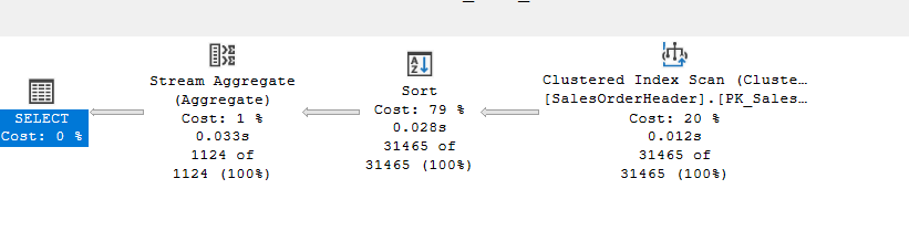

Now, if you compare the cost of each like:

The first was 0.793152
The second was 0.822284
The third was 2.73105

Since aggregating and sorting after that is way cheaper here, even though all of them produce the same output, again we explained all that before, but the point here, that these all could be hash or stream aggregates, regular ones, that if we want could interchange between each other if the optimizer estimate that they would be useful, and could even go parallel, unlike out upcoming operator

Now, how it does that?

Some traces and rules:

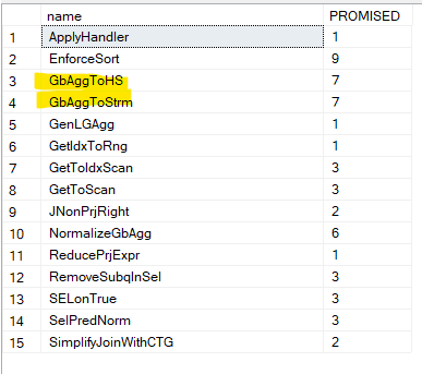
If we run some snapshots like we did before on sys.dm_exec_query_transformation_stats, we get two rules, We get these rules. Now there is no specific one here, it just generates two plans, one with stream aggregate that needs sorting like the last one, and one without, then it chooses the cheapest based on the estimates we showed before, and since sorting is expensive, it chooses to reduce its output by aggregating before.

We can see that here:

Root Group 21: Card=1124 (Max=34611.5, Min=0)

   7 <GbAggToHS>PhyOp_HashGbAgg 17.4 20.0  Cost(RowGoal 0,ReW 0,ReB 0,Dist 0,Total 0)= 0.793152 (Distance = 1)

   6 <EnforceSort>PhyOp_Sort 21.7  Cost(RowGoal 0,ReW 0,ReB 0,Dist 0,Total 0)= 0.822284 (Distance = 0)

   1 <GenLGAgg>LogOp_GbAgg 24 28 (Distance = 1)

   0 LogOp_GbAgg 17 20 (Distance = 0)

Here you can see that the first plan, without the order by before sorting, and since we wanted to enforce sort in the second query, it showed us just that

Now, if we compare that to the other rule, we don’t even see it in the memo, and the cost was not even calculated, now in the trace dumps I can’t see it, but the point being is, sorting 1000 is after aggregating 30 000, is way less than sorting 30 000 and aggregating them again.

ROLLUP

Now, there we just wanted a simple aggregation, sales by OrderDate, but what if we want the total sales as well, we can do this:

use adventureworks2022;
go
select OrderDate, sum(SalesOrderID) as how_many_sales
from Sales.SalesOrderHeader
group by OrderDate
union all
select null, sum(SalesOrderId) as total_sales
from Sales.SalesOrderHeader
go

We get:

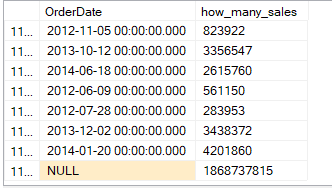
So, we get the total we want, but if we look at the execution plan:

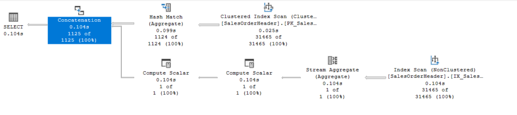
So here, it did what it did before in the upper section, aggregated, and then it went, aggregated again, we don’t see a sort because we have an index on SalesOrderId, now the first compute scalar is for outputting the sum as null if the sum = 0 since this is a scalar aggregate and it have to output something(for more on this check out this), and the second one is for the null that we selected, that does not belong anywhere,

and the concate is for the union all, nothing too fancy, but we see two aggregations, SQL Server has another way to reduce the cost of this, the group by rollup() syntax:

go
select OrderDate, sum(SalesOrderID) as how_many_sales
from Sales.SalesOrderHeader
group by rollup( OrderDate)
go

we get:

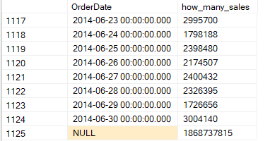
This null at the end represents our total, like we saw before, but if we look at the execution plan:

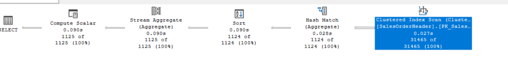
So we have the hash aggregate, like the one we saw before, nothing too fancy,

But we see a new stream aggregate, and since we can’t work with stream aggregate without sorting, we see the sort, what does that stream aggregate do:

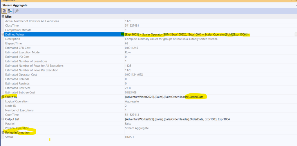
We see it is the rollup aggregate, and it has two sums, expr1005 and expr1006, which we get them from the hash aggregate properties, the 5 counts everything, the 6 counts the sums the sum

both sum both

But we see the rollup information:

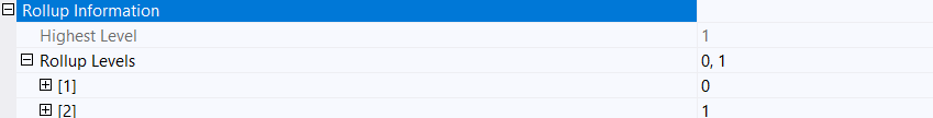
So we see the optimizer creating two levels, one by OrderDate, and the other by the whole table, not just OrderDate, meaning the scalar aggregate.

Now, this aggregate, is not like any other aggregate, it can’t be a hash aggregate, and it can’t have parallel plan, meaning it can’t apply the rules , or GenLGAgg rule to itself, but the hash could be a stream or parallel, like we showed before.

But we got rid of summing the whole thing aggregate, the lower section of the previous query.

The count here is the count in other aggregates, there to guarantee that the aggregate sum outputs null in the case of no rows.

So it does not do much, just sums once per group, then sums the total.

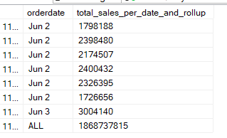
Now we can get rid of the null for total and replace it with any expression like all, since here it means the sum of all, like:

Using Grouping to get rid of nulls

go
select case when grouping(OrderDate) = 0
            then convert(char(5), orderdate)
            else 'ALL'
            end as orderdate,
            sum (salesorderid) as total_sales_per_date_and_rollup
from Sales.SalesOrderHeader 
group by rollup(OrderDate)
go

The output would be like:

Two columns in a rollup

What if we group by rollup by two columns like, meaning calculate totals per orderdate and SalesPersonId:

go
select OrderDate,SalesPersonID,sum(SalesOrderID)
from Sales.SalesOrderHeader
group by rollup(OrderDate,SalesPersonID)
go

We get:

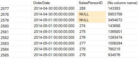
Now, here on 2014-04-30, it grouped the sum of SalesOrderId per SalesPersonId, then it calculated the total in the null, since there is no ALL concept in SQL Server. And the last null in the table is the sum of all SalesOrderId.

So different combinations with different order of columns, here you first process the dates and calculate their totals, if you reverse the order, you would calculate the SalesPersonId totals first per OrderDate

The execution plan:

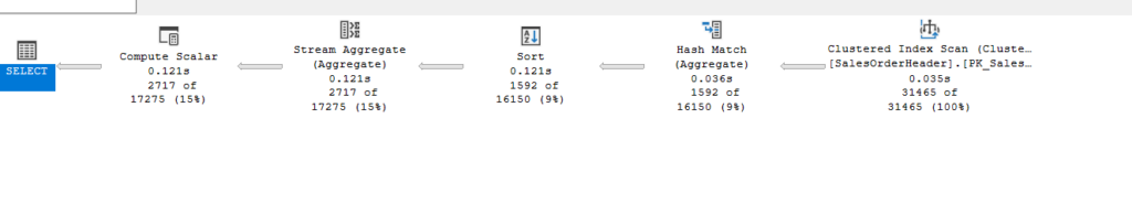
So, we see a similar plan if we look at the properties of the stream aggregate:

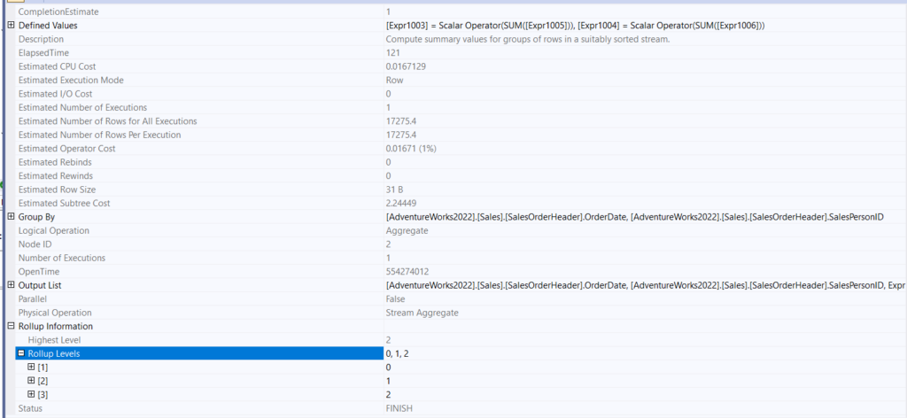
So, we see 3 different levels of rollup, it rolls up for each OrderDate SalesPersonID combination, then totals that specific date, then after that it gives us our total of totals.

The Expr1000 does not differ that much; one of them is there to prep for the occasion when there are no rows, and the other sums the hash aggregated values.

It also has different group by columns, so different columns, and different rollup levels.

We can replace nulls with the isnull here like:

go
select
case when grouping(OrderDate) = 0
     then convert(char(5),OrderDate)
     else 'ALL'
     end as OrderDate,
case when grouping(SalesPersonId) = 0
     then convert(char(5),SalesPersonId)
     else'ALL'
     end as SalePersonId,
sum(SalesOrderID),
GROUPING(OrderDate)as grouping_orderdate,
GROUPING(SalesPersonID) as grouping_salespersonid
from Sales.SalesOrderHeader
group by rollup(OrderDate,SalesPersonID)
go

We get the same execution plan. Here we know from the grouping, whether we are using that specific column to group by rollup or not, if we are, then 0, otherwise we get 1

The other nulls are not related to the group by rollup, they are actual nulls that we should see:

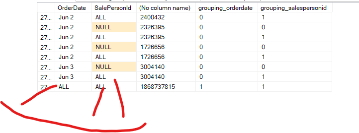
These ‘all’ values are the nulls from grouping, as we can see from the output of the grouping columns, the others are actual nulls.

Now if we want to look at the behind the scenes implementation of these in the optimizer:

Traces and rules

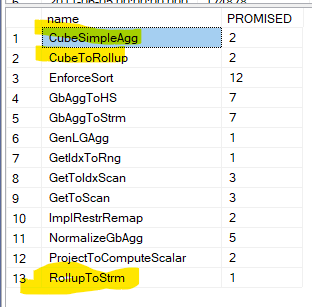
We can see the rules converting the rollup to a stream aggregate, the cube is another aggregation function that we are going to discuss in the next blog.

But when it starts, the rollup and the cube are both implemented as cube logical operator

Then, after that, if you asked for a rollup, it gets converted

And from there to a stream aggregate,

And from there we get a sort

If you ever wonder what the name of the logical operator of the rollup is:

DBCC execution completed. If DBCC printed error messages, contact your system administrator.
*** Converted Tree: ***
    LogOp_Project QCOL: [AdventureWorks2022].[Sales].[SalesOrderHeader].OrderDate COL: Expr1002 
       LogOp_Cube OUT(QCOL: [AdventureWorks2022].[Sales].[SalesOrderHeader].OrderDate,COL: Expr1002 ,) BY(QCOL: [AdventureWorks2022].[Sales].[SalesOrderHeader].OrderDate,) GROUPING SETS(0x0 0x1 )
            LogOp_Project
                LogOp_Project
                    LogOp_Get TBL: Sales.SalesOrderHeader Sales.SalesOrderHeader TableID=5f7e2dac TableReferenceID=0 IsRow: COL: IsBaseRow1000 
                    AncOp_PrjList 
                       ...........
                AncOp_PrjList 
            AncOp_PrjList 
                AncOp_PrjEl COL: Expr1002 
                    ScaOp_AggFunc stopSum Transformed
                        ScaOp_Identifier QCOL: [AdventureWorks2022].[Sales].[SalesOrderHeader].SalesOrderID
        AncOp_PrjList

Here, in the converted tree, in the binder, when the computed column still gets represented, that is the stuff we chose to omit here, we see the LogOp_Cube on order date, so they all start like that,

After that we have the sum(),

***** Rule applied: CubeSimpleAgg - Cube Simple Agg
--- tries to make the plan more optimizable
***** Rule applied: CubeToRollup - Cube Degenerate
---- like the name suggests, it converts the cube logical operator to a rollup
---- all this happens before simplificatio

And we end this blog here, catch you next time.

Resources:

Craig Freedman